
Nonlinear algebra#
KEYWORDS: scipy.optimize.fsolve, scipy.misc.derivative, list comprehension
Introduction to nonlinear algebra#
In non-linear algebra, we seek solutions to the equation \(f(x) = 0\) where \(f(x)\) is non-linear in \(x\). These are examples of non-linear algebraic equations:
\(e^x=4\)
\(x^2 + x - 1 = 0\)
\(f(F_A) = F_{A0} - F_{A} - k F_A^2 / \nu / V = 0\)
There is not a general theory for whether there is a solution, multiple solutions, or no solution to nonlinear algebraic equations. For example,
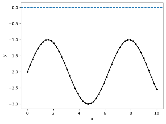
\(sin(x) = 2\) has no solution. We define \(f(x) = sin(x) - 2\) and plot it. You can see there no intersections with the x-axis at y=0, meaning no solutions.
import matplotlib.pyplot as plt
import numpy as np

x = np.linspace(0, 10)


def f(x):
    return np.sin(x) - 2


plt.plot(x, f(x), "k.-")
plt.axhline(0, ls="--")
plt.xlabel("x")
plt.ylabel("y");
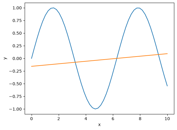
In contrast, \(sin(x) = 0.5\) will have an infinite number of solutions, everywhere the function intersects the x-axis.
def f2(x):
    return np.sin(x) - (x - 4)


# plt.plot(x, f2(x))
plt.plot(x, np.sin(x))
plt.plot(x, 0.025 * (x - 2 * np.pi))
# plt.axhline(0, ls='--')
plt.xlabel("x")
plt.ylabel("y");
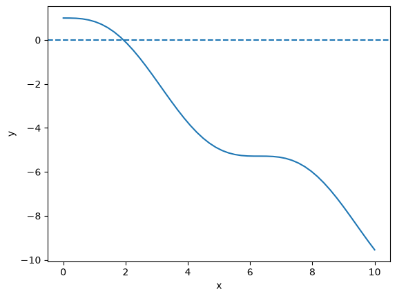
Finally, \(sin(x) = x - 1\) has only one solution.
def f3(x):
    return np.sin(x) - (x - 1)


plt.plot(x, f3(x))
plt.axhline(0, ls="--")
plt.xlabel("x")
plt.ylabel("y");
The equation \(e^{-0.5 x} \sin(x) = 0.5\), evidently has two solutions, but other versions of this equation might have 0, 1, multiple or infinite solutions.
def f3(x):
    return np.exp(-x) * np.sin(x) + 4000


x = np.linspace(-10, 6, 10000)
plt.plot(x, f3(x))
plt.axhline(0, ls="--")
# plt.title('$e^{-0.5 x} \sin(x) = 0.5$')
plt.xlabel("x")
plt.ylabel("objective")
plt.ylim([-5, 50]);
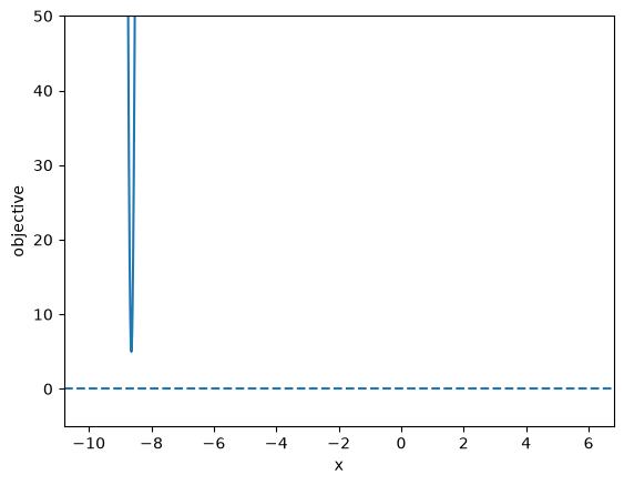
exercise modify the equation to see 0, 1, many or infinite solutions.
Graphical methods like this are invaluable to visually assess if there are any solutions, and if so how many solutions at least over some range of solutions. Sometimes, this is the fastest way to estimate a solution. Here we focus on nonlinear algebra problems that cannot be analytically solved. These kinds of problems require an iterative solution approach.
Newton-Raphson method for finding solutions#
Notes adapted from https://en.wikipedia.org/wiki/Newton%27s_method.
The key idea is that we start with a guess that is close to the solution, and then the function is approximated by a line tangent to the function to find where the line intersects the x-axis. For well-behaved functions, this is a better estimate of where the function equals zero than the first guess. Then, we repeat this until we get sufficiently close to zero.
So, we start with the point (x0, f(x0)), and we compute f’(x0), which is the slope of the line tangent to f(x0). We can express an equation for this line as: \(y - f(x0) = f'(x0)(x - x0)\) If we now solve this for the \(x\) where \(y=0\) leads to:
\(0 = f'(x0)(x - x0) + f(x0)\)
which leads to
\(x = x0 - f(x0) / f'(x0)\)
To implement this, we need to decide what is the tolerance for defining 0, and what is the maximum number of iterations we want to consider?
We will first consider what is the square root of 612? This is equivalent to finding a solution to \(x^2 = 612\)
\(f(x) = x^2 - 612\)
Let’s start with a guess of x=25, since we know \(x^2=625\). We also know \(f'(x) = 2x\).
The approach is iterative, so we will specify the maximum number of steps to iterate to, and a criteria for stopping.
x0 = 25


def f(x):
    return x**2 - 612


def fprime(x):
    return 2 * x


x = x0 - f(x0) / fprime(x0)
x, f(x), x**2
(24.74, 0.06759999999997035, 612.0676)
x = x - f(x) / fprime(x)
x, f(x), x**2
(24.738633791430882, 1.8665258494365844e-06, 612.0000018665258)
x0 = -0.25

Nmax = 25  # stop if we hit this many iterations
TOL = 1e-6  # stop if we are less than this number


def f(x):
    "The function to solve."
    return x**2 - 612


def fprime(x):
    "Derivative of the function to solve."
    return 2 * x


# Here is the iterative solution
for i in range(Nmax):
    xnew = x0 - f(x0) / fprime(x0)
    x0 = xnew

    print(f"{i}: {xnew}")
    if np.abs(f(xnew)) < TOL:
        break

    if i == Nmax - 1:
        print("Max iterations exceeded")
        break

print(xnew, xnew**2)
0: -1224.125
1: -612.3124744715614
2: -306.65598207645877
3: -154.3258518917108
4: -79.14574344693564
5: -43.43915671458881
6: -28.76391400152738
7: -25.020286679532415
8: -24.740219034714983
9: -24.738633804496054
10: -24.73863375370596
-24.73863375370596 611.9999999999999
That is pretty remarkable, it only took two iterations. That is partly because we started pretty close to the answer. Try this again with different initial guesses and see how the number of iterations changes. Also try with negative numbers. There are two solutions that are possible, and the one you get depends on the initial guess.
One reason it takes so few iterations here is that Newton’s method converges quadratically when you are close to the solution, and in this simple case we have a quadratic function, so we get to the answer in just a few steps.
Problem problems#
There are pathological situations you can get into. Consider this simple looking polynomial:
def f(x):
    return x**3 - 2 * x + 2


def fprime(x):
    return 3 * x**2 - 2


x = np.linspace(-2, 2)
plt.plot(x, f(x))
plt.xlabel("x")
plt.ylabel("f(x)");
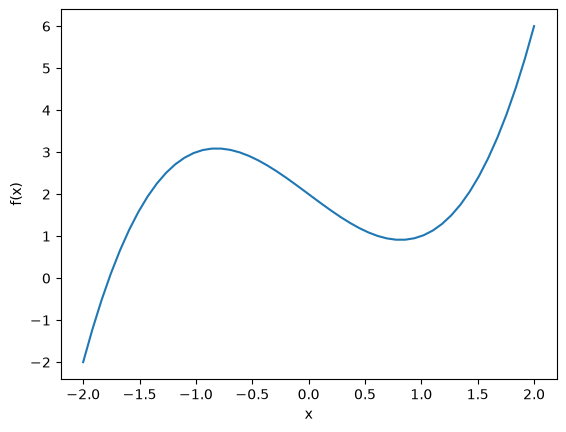
It seems obvious there is a root near -1.7. But if you use a guess around x=0, the algorithm simply oscillates back and forth and never converges. Let’s see:
x0 = 2

for i in range(Nmax):
    xnew = x0 - f(x0) / fprime(x0)
    x0 = xnew
    print(f"{i}: {xnew}  {f(x0)}  {fprime(x0)}")
    if np.abs(f(xnew)) < TOL:
        break

    if i == Nmax - 1:
        print("Max iterations exceeded")
        break

print(xnew)
0: 1.4  1.9439999999999995  3.879999999999999
1: 0.8989690721649484  0.9285595695281881  0.4244361781273245
2: -1.2887793276654596  2.4369578531870273  2.9828564662535015
3: -2.105767299013565  -3.1259765087015694  11.302767752784657
4: -1.8291999504602496  -0.46205275489156605  8.03791737629134
5: -1.771715812062107  -0.01794341645386366  7.416930756132674
6: -1.76929656115579  -3.1094202426196205e-05  7.391230963953113
7: -1.769292354251341  -9.39386346487936e-11  7.391186304436758
-1.769292354251341
Exercise: Try several initial guesses, and see which ones converge.
You can also run into problems when:
\(f'(x) = 0\) at the initial guess, or a subsequent unpdate, then you get a singularity in the update.
The first derivative is discontinuous at the root. Then you may not converge because the update can bounce back and forth.
The first derivative is undefined at the root
We do not frequently run into these issues, but they do occur from time to time. The solution is usually to use a better initial guess.
Derivatives of functions#
When you can derive an analytical derivative, you should probably consider doing that, because otherwise we have to approximate the derivatives numerically using finite differences, which is less accurate and computationally more expensive, or we need to use advance libraries that are capable of finding derivatives automatically. We will first see how to the finite differences approach, and later learn about the automatic approach.
Let’s examine the scipy.misc.derivative function. You provide a function, an x-value that you want the derivative at, and a dx to use in a finite-difference formula. By default, three points are used in the difference formula. You want to use a small dx to get an accurate result, but not too small or you can get numerical errors.
exercise: Try this out with different values of dx from 0.1 to 1e-15.
from scipy.misc import derivative
/tmp/ipykernel_2820/2127341723.py:1: DeprecationWarning: scipy.misc is deprecated and will be removed in 2.0.0
  from scipy.misc import derivative
---------------------------------------------------------------------------
ImportError                               Traceback (most recent call last)
Cell In[10], line 1
----> 1 from scipy.misc import derivative

ImportError: cannot import name 'derivative' from 'scipy.misc' (/opt/hostedtoolcache/Python/3.11.15/x64/lib/python3.11/site-packages/scipy/misc/__init__.py)
def f(x):
    return x**3


x0 = 12

derivative(f, x0, dx=1e-6), 3 * x0**2  # the numerical and analytical derivative
---------------------------------------------------------------------------
NameError                                 Traceback (most recent call last)
Cell In[11], line 7
      3
      4
      5 x0 = 12
      6
----> 7 derivative(f, x0, dx=1e-6), 3 * x0**2  # the numerical and analytical derivative

NameError: name 'derivative' is not defined
It would be nice to have some adaptive code that just does the right thing to find a dx adaptively. Here is an example:
def fprime(func, x0, dx=0.1, tolerance=1e-6, nmax=10):
    """Estimate the derivative of func at x0. dx is the initial spacing to use, and
    it will be adaptively made smaller to get the derivative accurately with a
    tolerance. nmax is the maximum number of divisions to make.

    """
    d0 = derivative(func, x0, dx=dx)
    for i in range(nmax):
        dx = dx / 2
        dnew = derivative(func, x0, dx=dx)
        if np.abs(d0 - dnew) <= tolerance:
            return dnew
        else:
            d0 = dnew

    # You only get here when the loop has completed and not returned a value
    print("Maximum number of divisions reached")
    return None
And, here is our derivative function in action:
def f(x):
    return x**3


fprime(f, 12)
---------------------------------------------------------------------------
NameError                                 Traceback (most recent call last)
Cell In[13], line 5
      1 def f(x):
      2     return x**3
      3
      4
----> 5 fprime(f, 12)

Cell In[12], line 7, in fprime(func, x0, dx, tolerance, nmax)
      3     it will be adaptively made smaller to get the derivative accurately with a
      4     tolerance. nmax is the maximum number of divisions to make.
      5
      6     """
----> 7     d0 = derivative(func, x0, dx=dx)
      8     for i in range(nmax):
      9         dx = dx / 2
     10         dnew = derivative(func, x0, dx=dx)

NameError: name 'derivative' is not defined
Let’s wrap the Newton method in a function too, using our fprime function to get the derivative.
def newton(func, x0, tolerance=1e-6, nmax=10):
    for i in range(nmax):
        xnew = x0 - func(x0) / fprime(func, x0)
        x0 = xnew
        if np.abs(func(xnew)) < tolerance:
            return xnew

    print("Max iterations exceeded")
    return None
Now, we have a pretty convenient way to solve equations:
def f(x):
    return x**2 - 612


newton(f, 25), np.sqrt(612)
---------------------------------------------------------------------------
NameError                                 Traceback (most recent call last)
Cell In[15], line 5
      1 def f(x):
      2     return x**2 - 612
      3
      4
----> 5 newton(f, 25), np.sqrt(612)

Cell In[14], line 3, in newton(func, x0, tolerance, nmax)
      1 def newton(func, x0, tolerance=1e-6, nmax=10):
      2     for i in range(nmax):
----> 3         xnew = x0 - func(x0) / fprime(func, x0)
      4         x0 = xnew
      5         if np.abs(func(xnew)) < tolerance:
      6             return xnew

Cell In[12], line 7, in fprime(func, x0, dx, tolerance, nmax)
      3     it will be adaptively made smaller to get the derivative accurately with a
      4     tolerance. nmax is the maximum number of divisions to make.
      5
      6     """
----> 7     d0 = derivative(func, x0, dx=dx)
      8     for i in range(nmax):
      9         dx = dx / 2
     10         dnew = derivative(func, x0, dx=dx)

NameError: name 'derivative' is not defined
This is the basic idea behind nonlinear algebra solvers. Similar to the ode solver we used, there are functions in scipy written to solve nonlinear equations. We consider these next.
fsolve#
scipy.optimize.fsolve is the main function we will use to solve nonlinear algebra problems. fsolve can be used with functions where you have the derivative, and where you don’t.
from scipy.optimize import fsolve
Let’s see the simplest example.
Solve \(e^x = 2\).
import numpy as np


def objective(x):
    return np.exp(x) - 2  # equal to zero at the solution


print(fsolve(objective, 2))
print(np.log(2))
ans = fsolve(objective, 2)
print(f"{float(ans):1.2f}")
[0.69314718]
0.6931471805599453
---------------------------------------------------------------------------
TypeError                                 Traceback (most recent call last)
Cell In[17], line 11
      7
      8 print(fsolve(objective, 2))
      9 print(np.log(2))
     10 ans = fsolve(objective, 2)
---> 11 print(f"{float(ans):1.2f}")

TypeError: only 0-dimensional arrays can be converted to Python scalars
Note that the result is an array. We can unpack the array with this syntax. Note the comma. Why a comma? it indicates to Python that the results should be unpacked into the variable in a special way, i.e. the first value of the result goes into the first variable. That is all there is in this case.
This is the preferred way to get the value of the solution into x:
(x,) = fsolve(objective, 2)
x
np.float64(0.6931471805599455)
Here are two checks on the answer.
objective(x), x - np.log(2)
(np.float64(4.440892098500626e-16), np.float64(2.220446049250313e-16))
You can get a lot more information by setting full output to 1. Note you have to assign 4 variables to the output in this case. That status will be 1 if it succeeds.
ans, info, status, msg = fsolve(objective, 2, full_output=1)
ans, info, status, msg
(array([0.69314718]),
 {'nfev': 12,
  'fjac': array([[-1.]]),
  'r': array([-2.00000148]),
  'qtf': array([-4.74713158e-10]),
  'fvec': array([4.4408921e-16])},
 1,
 'The solution converged.')
Here is an example with no solution, and a different status flag.
def objective2(x):
    return np.exp(x) + 2


results = fsolve(objective2, 2, full_output=1)
results
(array([-28.0696978]),
 {'nfev': 22,
  'fjac': array([[1.]]),
  'r': array([6.75011061e-13]),
  'qtf': array([2.]),
  'fvec': array([2.])},
 5,
 'The iteration is not making good progress, as measured by the \n improvement from the last ten iterations.')
(ans,) = results[0]
objective2(ans), np.abs(objective2(ans)) <= 1e-6
(np.float64(2.000000000000645), np.False_)
Note
scipy.optimize.root is preferred now.
A worked example#
We can integrate fsolve with a variety of other problems. For example, here is an integral equation we need to solve in engineering problems. The volume of a plug flow reactor can be defined by this equation: \(V = \int_{Fa(V=0)}^{Fa} \frac{1}{r_a} dFa\) where \(r_a\) is the rate law. Suppose we know the reactor volume is 100 L, the inlet concentration of A is 1 mol/L, the volumetric flow is 10 L/min, and \(r_a = -k Ca\), with \(k=0.23\) 1/min. What is the exit molar flow rate? We need to solve the following equation:
The equation to solve here is:
\(f(Fa) = 100 - \int_{Fa(V=0)}^{Fa} \frac{1}{-k Fa/\nu} dFa\).
import numpy as np
from scipy.integrate import quad
from scipy.optimize import fsolve

k = 0.23  # 1 / min
nu = 10.0  # L / min
Cao = 1.0  # mol / L
Fa0 = Cao * nu


def integrand(Fa):
    return -1.0 / (k * Fa / nu)


def objective(Fa):
    integral, err = quad(integrand, Fa0, Fa)
    return 100.0 - integral


objective(0.15 * Fa0), 0.15 * Fa0
(17.51652239626604, 1.5)
To make a plot, there is a subtlety. We cannot integrate an array of \(F_A\) values. Previously, we used a for loop to get around this. There is another syntax called list comprehension that we can also use:
[objective(fa) for fa in [0.01, 0.1, 1, 2]] # list comprehension
[-200.33718604270166,
 -100.22479069513437,
 -0.11239534756747105,
 30.024438589821685]
You can already see the answer must be between 1 and 2 because the sign changes between these two values, and that it is closer to 1 than 2.
import matplotlib.pyplot as plt

fa = np.linspace(0.01, Fa0)
obj = [objective(f) for f in fa]
plt.plot(fa, obj)
plt.xlabel("Molar flow rate (mol/min)")
plt.ylabel("objective")
plt.axhline(0, color="k", linestyle="--")
plt.axvline(1, color="k", linestyle="--");
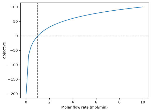
You can see there is one answer in this range, near a flow rate of 1.0 mol/min. We use that as an initial guess for fsolve:
Fa_guess = 1.0
(Fa_exit,) = fsolve(objective, Fa_guess)
print(f"The exit flow rate is {Fa_exit:1.4f} mol/min.")
---------------------------------------------------------------------------
TypeError                                 Traceback (most recent call last)
Cell In[26], line 2
      1 Fa_guess = 1.0
----> 2 (Fa_exit,) = fsolve(objective, Fa_guess)
      3 print(f"The exit flow rate is {Fa_exit:1.4f} mol/min.")

File /opt/hostedtoolcache/Python/3.11.15/x64/lib/python3.11/site-packages/scipy/optimize/_minpack_py.py:171, in fsolve(func, x0, args, fprime, full_output, col_deriv, xtol, maxfev, band, epsfcn, factor, diag)
    161 _wrapped_func.nfev = 0
    163 options = {'col_deriv': col_deriv,
    164            'xtol': xtol,
    165            'maxfev': maxfev,
   (...)    168            'factor': factor,
    169            'diag': diag}
--> 171 res = _root_hybr(_wrapped_func, x0, args, jac=fprime, **options)
    172 res.nfev = _wrapped_func.nfev
    174 if full_output:

File /opt/hostedtoolcache/Python/3.11.15/x64/lib/python3.11/site-packages/scipy/optimize/_minpack_py.py:239, in _root_hybr(func, x0, args, jac, col_deriv, xtol, maxfev, band, eps, factor, diag, **unknown_options)
    237 if not isinstance(args, tuple):
    238     args = (args,)
--> 239 shape, dtype = _check_func('fsolve', 'func', func, x0, args, n, (n,))
    240 if epsfcn is None:
    241     epsfcn = finfo(dtype).eps

File /opt/hostedtoolcache/Python/3.11.15/x64/lib/python3.11/site-packages/scipy/optimize/_minpack_py.py:24, in _check_func(checker, argname, thefunc, x0, args, numinputs, output_shape)
     22 def _check_func(checker, argname, thefunc, x0, args, numinputs,
     23                 output_shape=None):
---> 24     res = atleast_1d(thefunc(*((x0[:numinputs],) + args)))
     25     if (output_shape is not None) and (shape(res) != output_shape):
     26         if (output_shape[0] != 1):

File /opt/hostedtoolcache/Python/3.11.15/x64/lib/python3.11/site-packages/scipy/optimize/_minpack_py.py:159, in fsolve.<locals>._wrapped_func(*fargs)
    154 """
    155 Wrapped `func` to track the number of times
    156 the function has been called.
    157 """
    158 _wrapped_func.nfev += 1
--> 159 return func(*fargs)

Cell In[23], line 16, in objective(Fa)
     15 def objective(Fa):
---> 16     integral, err = quad(integrand, Fa0, Fa)
     17     return 100.0 - integral

File /opt/hostedtoolcache/Python/3.11.15/x64/lib/python3.11/site-packages/scipy/integrate/_quadpack_py.py:479, in quad(func, a, b, args, full_output, epsabs, epsrel, limit, points, weight, wvar, wopts, maxp1, limlst, complex_func)
    476     return retval
    478 if weight is None:
--> 479     retval = _quad(func, a, b, args, full_output, epsabs, epsrel, limit,
    480                    points)
    481 else:
    482     if points is not None:

File /opt/hostedtoolcache/Python/3.11.15/x64/lib/python3.11/site-packages/scipy/integrate/_quadpack_py.py:626, in _quad(func, a, b, args, full_output, epsabs, epsrel, limit, points)
    624 if points is None:
    625     if infbounds == 0:
--> 626         return _quadpack._qagse(func,a,b,args,full_output,epsabs,epsrel,limit)
    627     else:
    628         return _quadpack._qagie(func, bound, infbounds, args, full_output,
    629                                 epsabs, epsrel, limit)

TypeError: only 0-dimensional arrays can be converted to Python scalars
# Checking the answer different ways.
objective(Fa_exit), quad(integrand, Fa0, Fa_exit)
---------------------------------------------------------------------------
NameError                                 Traceback (most recent call last)
Cell In[27], line 2
      1 # Checking the answer different ways.
----> 2 objective(Fa_exit), quad(integrand, Fa0, Fa_exit)

NameError: name 'Fa_exit' is not defined
Parameterized objective functions#
Now, suppose we want to see how our solution varies with a parameter value. For example, we can change the rate constant by changing the temperature. Say we want to compute the exit molar flow rate at a range of rate constants, e.g. from 0.02 to 2 1/min. In other words, we treat the rate constant as a parameter and use it in an additional argument.
def integrand(Fa, k):
    return -1.0 / (k * Fa / nu)


def objective(Fa, k):
    integral, err = quad(integrand, Fa0, Fa, args=(k,))
    return 100.0 - integral


KRANGE = np.linspace(0.02, 2)

fa_exit = np.zeros(KRANGE.shape)

guess = 1.0

for i, k in enumerate(KRANGE):
    ans, info, status, msg = fsolve(objective, guess, args=(k,), full_output=1)
    if status == 1:
        fa_exit[i] = ans
        guess = ans
    else:
        print(f"k = {k} failed. {msg}")

X = (Fa0 - fa_exit) / Fa0
plt.plot(KRANGE, X, "b.-")
plt.xlabel("k (1/min)")
plt.ylabel("Conversion");
---------------------------------------------------------------------------
TypeError                                 Traceback (most recent call last)
Cell In[28], line 17
     13
     14 guess = 1.0
     15
     16 for i, k in enumerate(KRANGE):
---> 17     ans, info, status, msg = fsolve(objective, guess, args=(k,), full_output=1)
     18     if status == 1:
     19         fa_exit[i] = ans
     20         guess = ans

File /opt/hostedtoolcache/Python/3.11.15/x64/lib/python3.11/site-packages/scipy/optimize/_minpack_py.py:171, in fsolve(func, x0, args, fprime, full_output, col_deriv, xtol, maxfev, band, epsfcn, factor, diag)
    161 _wrapped_func.nfev = 0
    163 options = {'col_deriv': col_deriv,
    164            'xtol': xtol,
    165            'maxfev': maxfev,
   (...)    168            'factor': factor,
    169            'diag': diag}
--> 171 res = _root_hybr(_wrapped_func, x0, args, jac=fprime, **options)
    172 res.nfev = _wrapped_func.nfev
    174 if full_output:

File /opt/hostedtoolcache/Python/3.11.15/x64/lib/python3.11/site-packages/scipy/optimize/_minpack_py.py:239, in _root_hybr(func, x0, args, jac, col_deriv, xtol, maxfev, band, eps, factor, diag, **unknown_options)
    237 if not isinstance(args, tuple):
    238     args = (args,)
--> 239 shape, dtype = _check_func('fsolve', 'func', func, x0, args, n, (n,))
    240 if epsfcn is None:
    241     epsfcn = finfo(dtype).eps

File /opt/hostedtoolcache/Python/3.11.15/x64/lib/python3.11/site-packages/scipy/optimize/_minpack_py.py:24, in _check_func(checker, argname, thefunc, x0, args, numinputs, output_shape)
     22 def _check_func(checker, argname, thefunc, x0, args, numinputs,
     23                 output_shape=None):
---> 24     res = atleast_1d(thefunc(*((x0[:numinputs],) + args)))
     25     if (output_shape is not None) and (shape(res) != output_shape):
     26         if (output_shape[0] != 1):

File /opt/hostedtoolcache/Python/3.11.15/x64/lib/python3.11/site-packages/scipy/optimize/_minpack_py.py:159, in fsolve.<locals>._wrapped_func(*fargs)
    154 """
    155 Wrapped `func` to track the number of times
    156 the function has been called.
    157 """
    158 _wrapped_func.nfev += 1
--> 159 return func(*fargs)

Cell In[28], line 6, in objective(Fa, k)
      5 def objective(Fa, k):
----> 6     integral, err = quad(integrand, Fa0, Fa, args=(k,))
      7     return 100.0 - integral

File /opt/hostedtoolcache/Python/3.11.15/x64/lib/python3.11/site-packages/scipy/integrate/_quadpack_py.py:479, in quad(func, a, b, args, full_output, epsabs, epsrel, limit, points, weight, wvar, wopts, maxp1, limlst, complex_func)
    476     return retval
    478 if weight is None:
--> 479     retval = _quad(func, a, b, args, full_output, epsabs, epsrel, limit,
    480                    points)
    481 else:
    482     if points is not None:

File /opt/hostedtoolcache/Python/3.11.15/x64/lib/python3.11/site-packages/scipy/integrate/_quadpack_py.py:626, in _quad(func, a, b, args, full_output, epsabs, epsrel, limit, points)
    624 if points is None:
    625     if infbounds == 0:
--> 626         return _quadpack._qagse(func,a,b,args,full_output,epsabs,epsrel,limit)
    627     else:
    628         return _quadpack._qagie(func, bound, infbounds, args, full_output,
    629                                 epsabs, epsrel, limit)

TypeError: only 0-dimensional arrays can be converted to Python scalars
You can see here that any rate constant above about 0.5 1/min leads to near complete conversion, so heating above the temperature required for this would be wasteful.
Summary#
In this lecture we reviewed methods to solve non-linear algebraic equations (they also work on linear algebra, but it is considered wasteful since there are more efficient methods to solve those).
The key idea is to create a function that is equal to zero at the solution, and then use
scipy.optimize.fsolvewith an initial guess to find the solution.We introduced list comprehension which is a convenient syntax for for loops.
We also looked at
scipy.misc.derivativewhich is a convenient way to numerically estimate the derivative of a function by finite difference formulas.