Neural Networks and Hyperparameter Tuning

Neural Networks and Hyperparameter Tuning#

Building flexible nonlinear models and tuning them systematically.

Learning Objectives#

Build and configure neural network regressors using sklearn’s MLPRegressor
Understand the role of key hyperparameters (hidden layers, activation, alpha, learning rate)
Use RandomizedSearchCV for efficient hyperparameter search over large spaces
Apply advanced cross-validation strategies (RepeatedKFold) for robust model evaluation
Compare nonlinear methods (polynomial, SVR, neural network, random forest) on a single problem

import numpy as np
import pandas as pd
import matplotlib.pyplot as plt
import time
import warnings
warnings.filterwarnings("ignore", category=UserWarning)

from sklearn.neural_network import MLPRegressor
from sklearn.ensemble import RandomForestRegressor
from sklearn.linear_model import LinearRegression, Ridge
from sklearn.preprocessing import PolynomialFeatures, StandardScaler
from sklearn.svm import SVR
from sklearn.model_selection import (
    train_test_split, cross_val_score,
    GridSearchCV, RandomizedSearchCV,
    KFold, RepeatedKFold
)
from sklearn.pipeline import Pipeline
from sklearn.metrics import mean_squared_error, r2_score
from scipy.stats import uniform, loguniform, randint

Neural Networks with sklearn#

Why Neural Networks?#

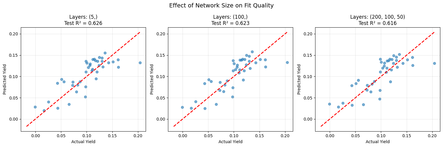
Neural networks are universal approximators: given enough neurons, they can model any continuous function to arbitrary accuracy. This makes them extremely flexible nonlinear models.

In chemical engineering, relationships between process variables are often complex and unknown. Neural networks can learn these relationships directly from data, without specifying the functional form.

How MLPRegressor Works#

The Multi-Layer Perceptron (MLP) passes inputs through layers of neurons:

Input layer: Receives the features (temperature, pressure, etc.)
Hidden layers: Apply nonlinear transformations (the “learning” happens here)
Output layer: Produces the prediction

Each neuron computes: \(z = \text{activation}(w_1 x_1 + w_2 x_2 + \ldots + b)\)

Training uses backpropagation: compute the error, propagate gradients backward through the network, and update weights to reduce the error. This is gradient descent applied to a network of nonlinear functions.

Key Hyperparameters#

Parameter	Controls	Typical Values
`hidden_layer_sizes`	Network architecture (depth & width)	(50,), (100, 50), (100, 50, 25)
`activation`	Nonlinear function at each neuron	relu, tanh, logistic
`alpha`	L2 regularization strength	0.0001 to 1.0
`learning_rate_init`	Step size for weight updates	0.001 to 0.01
`max_iter`	Maximum training epochs	200 to 2000
`early_stopping`	Stop when validation score stops improving	True/False
`solver`	Optimization algorithm	adam, lbfgs

# Load reaction yield dataset (temperature, pressure -> yield)
url = "https://raw.githubusercontent.com/jkitchin/s26-06642/main/dsmles/data/reaction_yield.csv"
df = pd.read_csv(url)

X = df[["temperature", "pressure"]].values
y = df["yield"].values

X_train, X_test, y_train, y_test = train_test_split(X, y, test_size=0.2, random_state=42)

print(f"Dataset: {X.shape[0]} samples, {X.shape[1]} features")
print(f"Training: {X_train.shape[0]}, Test: {X_test.shape[0]}")
df.describe()

Dataset: 200 samples, 2 features
Training: 160, Test: 40

	temperature	pressure	yield
count	200.000000	200.000000	200.000000
mean	396.801247	5.539376	0.099662
std	58.978286	2.637011	0.044511
min	301.104423	1.045554	-0.017316
25%	345.716483	3.353163	0.071893
50%	398.897251	5.874759	0.106432
75%	451.371923	7.679794	0.133522
max	497.377387	9.914546	0.204139

# Basic MLPRegressor - always use a Pipeline with StandardScaler!
nn_pipeline = Pipeline([
    ("scaler", StandardScaler()),
    ("mlp", MLPRegressor(hidden_layer_sizes=(20,), activation='tanh', solver='lbfgs', max_iter=1000, random_state=42))
])

nn_pipeline.fit(X_train, y_train)

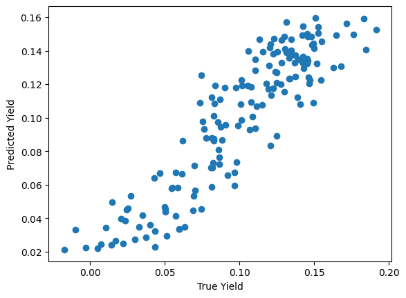
print(f"Training R²: {nn_pipeline.score(X_train, y_train):.4f}")
print(f"Test R²:     {nn_pipeline.score(X_test, y_test):.4f}")

plt.plot(y_train, nn_pipeline.predict(X_train), "o", label="Train")
plt.xlabel("True Yield")
plt.ylabel("Predicted Yield");

Training R²: 0.8193
Test R²:     0.6336

../_images/c748b84139810b2e5f5e19c8ff20dd463593ae2e2fc6d3e993d8232e050a7eca.png

Effect of Hidden Layer Size#

The hidden_layer_sizes parameter controls the network’s capacity:

Too small (e.g., (5,)): Not enough neurons to capture the relationship → underfitting
Just right (e.g., (50,) or (100,)): Captures the pattern without memorizing noise
Too large (e.g., (500, 500)): Can memorize training data → overfitting

The tuple format specifies layers: (100, 50) means first hidden layer has 100 neurons, second has 50.

# Compare different hidden layer sizes
architectures = {
    "(5,)": (5,),
    "(50,)": (50,),
    "(100,)": (100,),
    "(100, 50)": (100, 50),
    "(200, 100, 50)": (200, 100, 50),
}

results = []
for name, layers in architectures.items():
    pipe = Pipeline([
        ("scaler", StandardScaler()),
        ("mlp", MLPRegressor(hidden_layer_sizes=layers, activation='tanh', solver='lbfgs', max_iter=1000, random_state=42))
    ])
    pipe.fit(X_train, y_train)
    results.append({
        "Architecture": name,
        "Train R²": pipe.score(X_train, y_train),
        "Test R²": pipe.score(X_test, y_test),
        "# Parameters": sum(c.size for c in pipe.named_steps["mlp"].coefs_) +
                        sum(b.size for b in pipe.named_steps["mlp"].intercepts_)
    })

results_df = pd.DataFrame(results)
print(results_df.to_string(index=False))

  Architecture  Train R²  Test R²  # Parameters
          (5,)  0.828414 0.625546            21
         (50,)  0.834900 0.656535           201
        (100,)  0.826104 0.623063           401
     (100, 50)  0.832786 0.671971          5401
(200, 100, 50)  0.823373 0.615981         25801

# Visualize: predicted vs actual for small, medium, large networks
fig, axes = plt.subplots(1, 3, figsize=(15, 5))

for ax, (name, layers) in zip(axes, [("(5,)", (5,)), ("(100,)", (100,)), ("(200, 100, 50)", (200, 100, 50))]):
    pipe = Pipeline([
        ("scaler", StandardScaler()),
        ("mlp", MLPRegressor(hidden_layer_sizes=layers, 
                             solver='lbfgs', activation='tanh',
                             max_iter=1000, random_state=42))
    ])
    pipe.fit(X_train, y_train)
    y_pred = pipe.predict(X_test)
    
    ax.scatter(y_test, y_pred, alpha=0.6)
    ax.plot([y.min(), y.max()], [y.min(), y.max()], "r--", linewidth=2)
    ax.set_xlabel("Actual Yield")
    ax.set_ylabel("Predicted Yield")
    ax.set_title(f"Layers: {name}\nTest R² = {r2_score(y_test, y_pred):.3f}")
    ax.grid(True, alpha=0.3)

plt.suptitle("Effect of Network Size on Fit Quality", fontsize=14)
plt.tight_layout()
plt.show()

../_images/86f3a3d3526583b1da3e93750ec007b1f2a23948a23992daa067fb1b9c6f1ebb.png

Activation Functions#

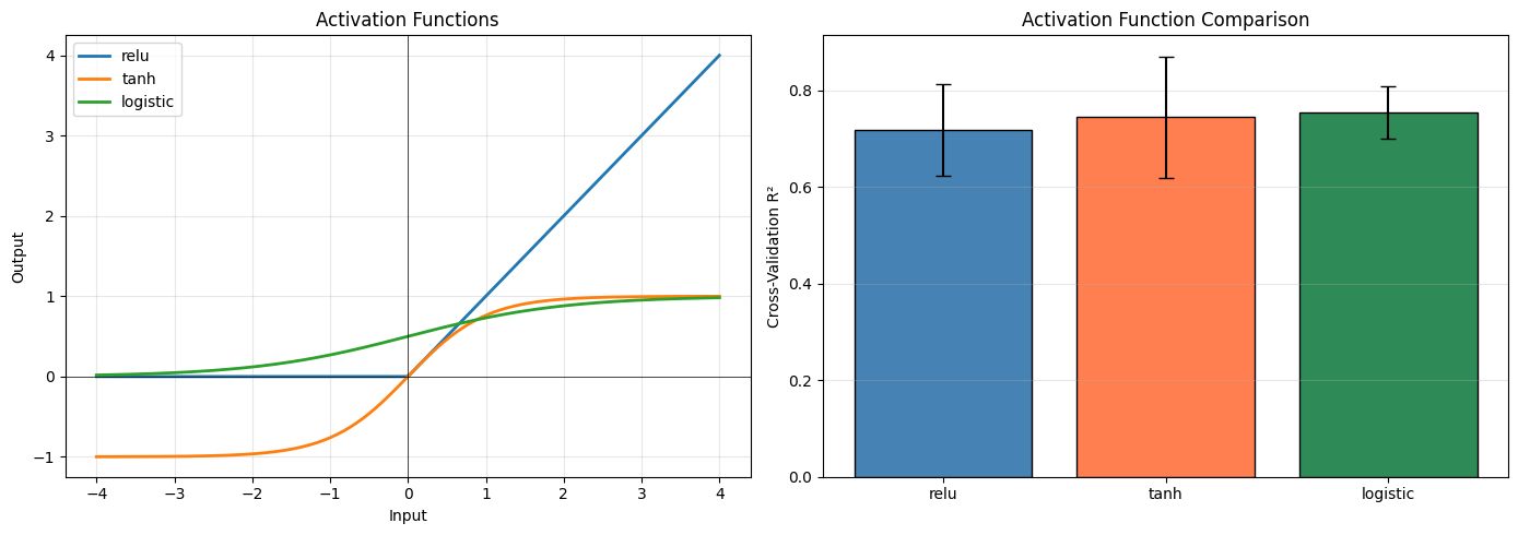
The activation function determines the nonlinear transformation at each neuron:

Function	Formula	Properties
relu	\(\max(0, x)\)	Fast, default choice, can “die” (output 0)
tanh	\(\tanh(x)\)	Output in [-1, 1], zero-centered
logistic	\(1/(1 + e^{-x})\)	Output in [0, 1], sigmoid shape

# Compare activation functions
fig, axes = plt.subplots(1, 2, figsize=(14, 5))

# Left: visualize the functions
x_act = np.linspace(-4, 4, 200)
axes[0].plot(x_act, np.maximum(0, x_act), label="relu", linewidth=2)
axes[0].plot(x_act, np.tanh(x_act), label="tanh", linewidth=2)
axes[0].plot(x_act, 1 / (1 + np.exp(-x_act)), label="logistic", linewidth=2)
axes[0].set_xlabel("Input")
axes[0].set_ylabel("Output")
axes[0].set_title("Activation Functions")
axes[0].legend()
axes[0].grid(True, alpha=0.3)
axes[0].axhline(y=0, color="black", linewidth=0.5)
axes[0].axvline(x=0, color="black", linewidth=0.5)

# Right: compare performance
activation_scores = []
for act in ["relu", "tanh", "logistic"]:
    pipe = Pipeline([
        ("scaler", StandardScaler()),
        ("mlp", MLPRegressor(hidden_layer_sizes=(100,), activation=act,
                             solver='lbfgs',
                             max_iter=1000, random_state=42))
    ])
    scores = cross_val_score(pipe, X, y, cv=5, scoring="r2")
    activation_scores.append({"Activation": act, "Mean CV R²": scores.mean(), "Std": scores.std()})

act_df = pd.DataFrame(activation_scores)
axes[1].bar(act_df["Activation"], act_df["Mean CV R²"], yerr=act_df["Std"] * 2,
            capsize=5, edgecolor="black", color=["steelblue", "coral", "seagreen"])
axes[1].set_ylabel("Cross-Validation R²")
axes[1].set_title("Activation Function Comparison")
axes[1].grid(True, alpha=0.3, axis="y")

plt.tight_layout()
plt.show()

../_images/588e34c3169bb84a6236785137395c50ed46d9bb61330d05f403a01b1e7c8c9c.png

Feature Scaling is Essential#

Neural networks use gradient-based optimization. If features have very different scales (e.g., temperature in hundreds, pressure in single digits), gradients become unbalanced and training fails or converges very slowly.

Always use StandardScaler in a Pipeline — this is the same requirement as SVR (Module 09) and regularized regression (Module 08). The pipeline ensures scaling is applied correctly during cross-validation without data leakage.

# What happens without scaling?
nn_no_scale = MLPRegressor(hidden_layer_sizes=(100,), max_iter=1000, random_state=42)
nn_no_scale.fit(X_train, y_train)

nn_with_scale = Pipeline([
    ("scaler", StandardScaler()),
    ("mlp", MLPRegressor(hidden_layer_sizes=(100,), 
                         activation='tanh',
                         solver='lbfgs',
                         max_iter=1000, random_state=42))
])
nn_with_scale.fit(X_train, y_train)

print("Without scaling:")
print(f"  Train R²: {nn_no_scale.score(X_train, y_train):.4f}")
print(f"  Test R²:  {nn_no_scale.score(X_test, y_test):.4f}")
print(f"\nWith scaling:")
print(f"  Train R²: {nn_with_scale.score(X_train, y_train):.4f}")
print(f"  Test R²:  {nn_with_scale.score(X_test, y_test):.4f}")
print(f"\nScaling improved test R² by {nn_with_scale.score(X_test, y_test) - nn_no_scale.score(X_test, y_test):.4f}")

Without scaling:
  Train R²: -33507.9439
  Test R²:  -41198.6360

With scaling:
  Train R²: 0.8261
  Test R²:  0.6231

Scaling improved test R² by 41199.2591

nn_with_scale

Pipeline(steps=[('scaler', StandardScaler()),
                ('mlp',
                 MLPRegressor(activation='tanh', max_iter=1000, random_state=42,
                              solver='lbfgs'))])

In a Jupyter environment, please rerun this cell to show the HTML representation or trust the notebook.
On GitHub, the HTML representation is unable to render, please try loading this page with nbviewer.org.

Alpha: L2 Regularization#

The alpha parameter in MLPRegressor is L2 regularization — the same concept as Ridge regression from Module 08. It penalizes large weights to prevent overfitting:

Small alpha (e.g., 0.0001): Minimal regularization, network can fit complex patterns (risk of overfitting)
Large alpha (e.g., 1.0): Strong regularization, simpler model (risk of underfitting)

Solver Choice#

adam: Good default for most problems. Adaptive learning rate, handles noise well.
lbfgs: Quasi-Newton method. Works well on small datasets (<1000 samples). Deterministic.

Early Stopping#

Set early_stopping=True to automatically stop training when validation performance stops improving. This is a practical way to prevent overfitting without manually choosing max_iter.

# Effect of alpha (L2 regularization)
alphas = [0.0001, 0.001, 0.01, 0.1, 1.0, 10.0]
alpha_results = []

for alpha in alphas:
    pipe = Pipeline([
        ("scaler", StandardScaler()),
        ("mlp", MLPRegressor(hidden_layer_sizes=(100, 50), alpha=alpha,
                             max_iter=1000, random_state=42))
    ])
    pipe.fit(X_train, y_train)
    alpha_results.append({
        "alpha": alpha,
        "Train R²": pipe.score(X_train, y_train),
        "Test R²": pipe.score(X_test, y_test)
    })

alpha_df = pd.DataFrame(alpha_results)

plt.figure(figsize=(10, 6))
plt.semilogx(alpha_df["alpha"], alpha_df["Train R²"], "o-", label="Train R²")
plt.semilogx(alpha_df["alpha"], alpha_df["Test R²"], "s-", label="Test R²")
plt.xlabel("Alpha (L2 Regularization)")
plt.ylabel("R²")
plt.title("Effect of Alpha on MLPRegressor (like Ridge for neural networks)")
plt.legend()
plt.grid(True, alpha=0.3)
plt.show()

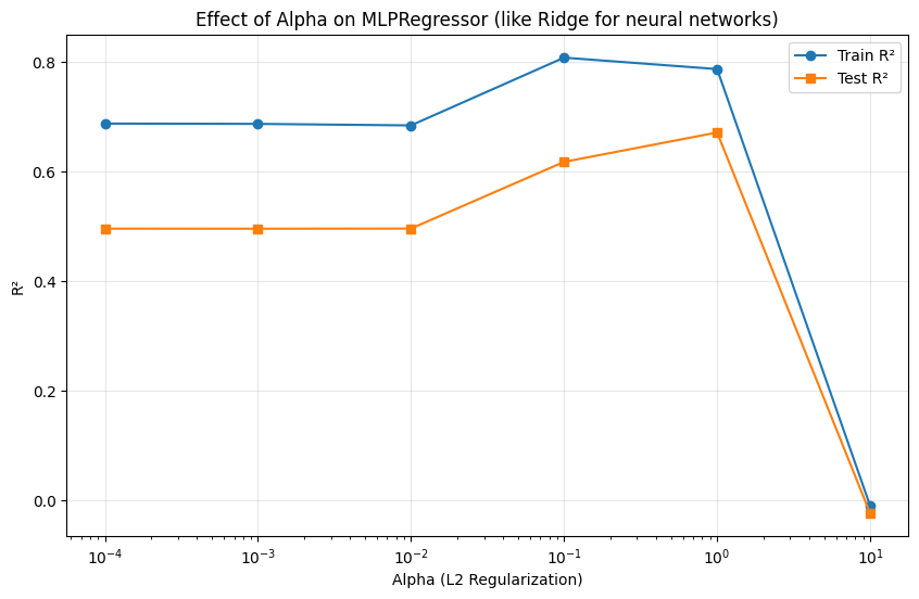
../_images/81f9c4e68cb78a4e1dbdc13089df24f22f081480f57e7fbc55e2104788f0f2e3.png

Hyperparameter tuning can be essential to getting a good and useful model.

Random Forest Preview#

Before Module 10 covers ensemble methods in depth, let’s preview Random Forests — one of the most practical and widely-used nonlinear methods.

From Trees to Forests#

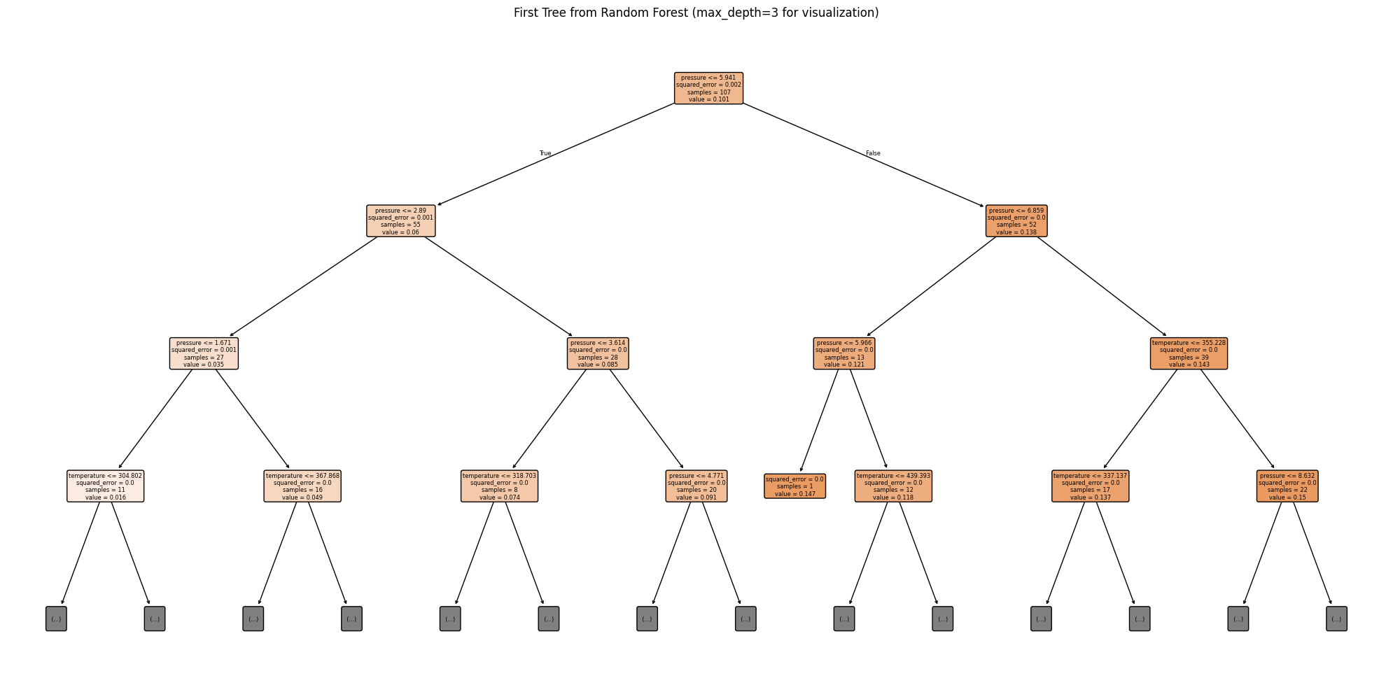
A decision tree splits data using yes/no questions (e.g., “Is temperature > 400K?”). At each leaf node, it predicts the average of the training points that landed there. Trees naturally handle nonlinearity — each split creates a piecewise-constant approximation.

The problem: individual trees are unstable and prone to overfitting. Small changes in the training data can produce very different trees.

A Random Forest fixes this by:

Training many trees on random subsets of the data (bootstrap sampling)
Using random subsets of features at each split
Averaging all predictions

This reduces variance dramatically while maintaining the flexibility of trees.

Key Hyperparameters#

Parameter	Effect	Typical Range
`n_estimators`	Number of trees (more is better, just slower)	100-500
`max_depth`	Maximum tree depth (controls complexity)	5-20 or None
`min_samples_split`	Minimum samples to split a node	2-10
`max_features`	Features considered at each split	“sqrt”, “log2”, or fraction

No Scaling Required#

Unlike neural networks and SVR, Random Forests do not need feature scaling. Tree splits depend on thresholds, not distances or gradients, so the absolute scale of features doesn’t matter.

# Random Forest on the same dataset — no scaling needed!
rf = RandomForestRegressor(n_estimators=100, max_depth=10, random_state=42, n_jobs=-1)
rf.fit(X_train, y_train)

print("Random Forest (no scaling):")
print(f"  Train R²: {rf.score(X_train, y_train):.4f}")
print(f"  Test R²:  {rf.score(X_test, y_test):.4f}")

# Compare with our neural network
nn_pipe = Pipeline([
    ("scaler", StandardScaler()),
    ("mlp", MLPRegressor(hidden_layer_sizes=(100,), max_iter=1000, random_state=42))
])
nn_pipe.fit(X_train, y_train)

print(f"\nNeural Network (with scaling):")
print(f"  Train R²: {nn_pipe.score(X_train, y_train):.4f}")
print(f"  Test R²:  {nn_pipe.score(X_test, y_test):.4f}")

print("\nRandom Forest works well out of the box with minimal tuning!")
print("Module 10 covers ensemble methods (Random Forests, Gradient Boosting, XGBoost) in depth.")

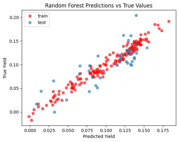
Random Forest (no scaling):
  Train R²: 0.9669
  Test R²:  0.6441

Neural Network (with scaling):
  Train R²: -1.0961
  Test R²:  -1.4254

Random Forest works well out of the box with minimal tuning!
Module 10 covers ensemble methods (Random Forests, Gradient Boosting, XGBoost) in depth.

plt.plot(rf.predict(X_train), y_train, "ro", label="train", alpha=0.6)
plt.plot(rf.predict(X_test), y_test, "o", label="test", alpha=0.6)
plt.xlabel("Predicted Yield")
plt.ylabel("True Yield")
plt.title("Random Forest Predictions vs True Values")
plt.legend();

../_images/96669d3b72e143cb1ee587838c76e3425bc0e2ce6417042747590c4f26956ee9.png

rf

RandomForestRegressor(max_depth=10, n_jobs=-1, random_state=42)

In a Jupyter environment, please rerun this cell to show the HTML representation or trust the notebook.
On GitHub, the HTML representation is unable to render, please try loading this page with nbviewer.org.

from sklearn.tree import plot_tree

# Visualize the first tree in the random forest
plt.figure(figsize=(20, 10))
plot_tree(rf.estimators_[0], 
          feature_names=df.columns[:-1],  # All columns except the last (target)
          filled=True, 
          rounded=True,
          max_depth=3)  # Limit depth for readability
plt.title("First Tree from Random Forest (max_depth=3 for visualization)")
plt.tight_layout()
plt.show()

../_images/faac59dec18c5ea3f3e798f2f3701f017628c1192018d20eb746270285dcf3c2.png

Hyperparameter Tuning Strategies#

The Challenge#

Neural networks have many hyperparameters that interact in complex ways. The difference between a poorly tuned and well-tuned neural network can be enormous — often larger than the difference between algorithm choices.

GridSearchCV Review#

We used GridSearchCV in the previous lecture to tune SVR. It tries every combination on a predefined grid:

param_grid = {"C": [0.1, 1, 10], "gamma": [0.01, 0.1, 1]}  # 9 combinations

Problem: With many hyperparameters, the grid grows exponentially. If you have 5 parameters with 5 values each, that’s \(5^5 = 3{,}125\) combinations, each requiring full cross-validation.

RandomizedSearchCV: A Smarter Approach#

Instead of trying every combination, sample randomly from the hyperparameter space:

Define probability distributions for each parameter
Sample n_iter random combinations
Evaluate each with cross-validation
Return the best

Why random search often beats grid search (Bergstra & Bengio, 2012):

Grid search wastes evaluations on unimportant parameters
If only 1-2 parameters really matter, random search explores more unique values of those parameters
You control the compute budget directly with n_iter

Choosing Distributions#

Use scipy.stats distributions for continuous hyperparameters:

Parameter Type	Distribution	Example
Log-scale (alpha, learning rate)	`loguniform(a, b)`	`loguniform(1e-5, 1e-1)`
Linear-scale (layer sizes)	`randint(a, b)`	`randint(10, 200)`
Bounded continuous	`uniform(loc, scale)`	`uniform(0, 1)`
Categorical	list	`["relu", "tanh"]`

# RandomizedSearchCV for MLPRegressor
pipeline = Pipeline([
    ("scaler", StandardScaler()),
    ("mlp", MLPRegressor(max_iter=1000, early_stopping=True, random_state=42))
])

# Define distributions for each hyperparameter
param_distributions = {
    "mlp__hidden_layer_sizes": [(50,), (100,), (50, 25), (100, 50), (100, 50, 25)],
    "mlp__activation": ["relu", "tanh"],
    "mlp__alpha": loguniform(1e-5, 1e-1),
    "mlp__learning_rate_init": loguniform(1e-4, 1e-2),
}

# Random search with 30 iterations (instead of exhaustive grid)
random_search = RandomizedSearchCV(
    pipeline,
    param_distributions,
    n_iter=30,
    cv=5,
    scoring="r2",
    random_state=42,
    n_jobs=-1
)

random_search.fit(X_train, y_train)

print("RandomizedSearchCV Results:")
print(f"  Best parameters: {random_search.best_params_}")
print(f"  Best CV R²: {random_search.best_score_:.4f}")
print(f"  Test R²: {random_search.score(X_test, y_test):.4f}")

RandomizedSearchCV Results:
  Best parameters: {'mlp__activation': 'tanh', 'mlp__alpha': np.float64(0.0017912362571043657), 'mlp__hidden_layer_sizes': (100,), 'mlp__learning_rate_init': np.float64(0.0004066563313514797)}
  Best CV R²: 0.7452
  Test R²: 0.6139

# Compare: GridSearchCV vs RandomizedSearchCV
# Grid search with a smaller, discrete grid
param_grid = {
    "mlp__hidden_layer_sizes": [(50,), (100,), (100, 50)],
    "mlp__activation": ["relu", "tanh"],
    "mlp__alpha": [0.0001, 0.001, 0.01, 0.1],
    "mlp__learning_rate_init": [0.001, 0.01],
}

grid_pipeline = Pipeline([
    ("scaler", StandardScaler()),
    ("mlp", MLPRegressor(max_iter=1000, early_stopping=True, random_state=42))
])

start = time.time()
grid_search = GridSearchCV(grid_pipeline, param_grid, cv=5, scoring="r2", n_jobs=-1)
grid_search.fit(X_train, y_train)
grid_time = time.time() - start

n_grid_combos = 1
for v in param_grid.values():
    n_grid_combos *= len(v)

print(f"GridSearchCV: {n_grid_combos} combinations, {grid_time:.1f}s")
print(f"  Best CV R²: {grid_search.best_score_:.4f}")
print(f"  Test R²:    {grid_search.score(X_test, y_test):.4f}")
print(f"\nRandomizedSearchCV: 30 iterations (from previous cell)")
print(f"  Best CV R²: {random_search.best_score_:.4f}")
print(f"  Test R²:    {random_search.score(X_test, y_test):.4f}")
print(f"\nRandom search explored 30 combinations vs Grid's {n_grid_combos}")

GridSearchCV: 48 combinations, 10.0s
  Best CV R²: 0.7714
  Test R²:    0.7046

RandomizedSearchCV: 30 iterations (from previous cell)
  Best CV R²: 0.7452
  Test R²:    0.6139

Random search explored 30 combinations vs Grid's 48

Cross-Validation Strategies#

The default cv=5 in scikit-learn uses KFold — split data into 5 parts, test on each. But a single 5-fold split can give different results depending on how the data was partitioned.

RepeatedKFold#

RepeatedKFold repeats K-fold cross-validation multiple times with different random splits, then averages all scores. This reduces the variance of the CV estimate:

cv = RepeatedKFold(n_splits=5, n_repeats=3, random_state=42)  # 15 total fits

n_splits=5, n_repeats=1: Standard 5-fold (5 fits)
n_splits=5, n_repeats=3: Three repetitions (15 fits) — more stable estimate
n_splits=5, n_repeats=10: Very stable estimate (50 fits) — useful for small datasets

When to use RepeatedKFold:

Small datasets where fold composition matters more
When comparing models with similar performance (need precise estimates)
When you want confidence in your CV score

Note: For classification, RepeatedStratifiedKFold maintains class balance in each fold. For regression, shuffling in KFold is what matters.

# Compare CV score stability: KFold vs RepeatedKFold
pipe = Pipeline([
    ("scaler", StandardScaler()),
    ("mlp", MLPRegressor(hidden_layer_sizes=(100,), max_iter=1000, random_state=42))
])

# Standard 5-fold (different random seeds give different scores)
kfold_scores_by_seed = []
for seed in range(10):
    cv = KFold(n_splits=5, shuffle=True, random_state=seed)
    scores = cross_val_score(pipe, X, y, cv=cv, scoring="r2")
    kfold_scores_by_seed.append(scores.mean())

# RepeatedKFold (inherently more stable)
cv_repeated = RepeatedKFold(n_splits=5, n_repeats=3, random_state=42)
repeated_scores = cross_val_score(pipe, X, y, cv=cv_repeated, scoring="r2")

print("Variability of 5-Fold CV across 10 different random splits:")
print(f"  Mean of means: {np.mean(kfold_scores_by_seed):.4f}")
print(f"  Std of means:  {np.std(kfold_scores_by_seed):.4f}")
print(f"  Range: [{np.min(kfold_scores_by_seed):.4f}, {np.max(kfold_scores_by_seed):.4f}]")

print(f"\nRepeatedKFold (5 splits x 3 repeats = 15 scores):")
print(f"  Mean: {repeated_scores.mean():.4f}")
print(f"  Std:  {repeated_scores.std():.4f}")
print(f"\nRepeatedKFold gives a single, more reliable estimate.")

Variability of 5-Fold CV across 10 different random splits:
  Mean of means: -1.5013
  Std of means:  0.0568
  Range: [-1.5853, -1.3956]

RepeatedKFold (5 splits x 3 repeats = 15 scores):
  Mean: -1.5408
  Std:  0.8292

RepeatedKFold gives a single, more reliable estimate.

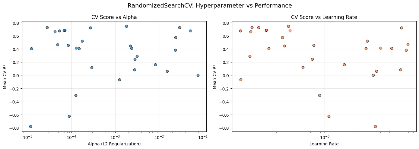
# Visualize RandomizedSearchCV results
results = pd.DataFrame(random_search.cv_results_)

fig, axes = plt.subplots(1, 2, figsize=(14, 5))

# Left: score vs alpha (log scale)
axes[0].scatter(results["param_mlp__alpha"].astype(float),
               results["mean_test_score"], alpha=0.7, edgecolors="black")
axes[0].set_xscale("log")
axes[0].set_xlabel("Alpha (L2 Regularization)")
axes[0].set_ylabel("Mean CV R²")
axes[0].set_title("CV Score vs Alpha")
axes[0].grid(True, alpha=0.3)

# Right: score vs learning rate (log scale)
axes[1].scatter(results["param_mlp__learning_rate_init"].astype(float),
               results["mean_test_score"], alpha=0.7, edgecolors="black", color="coral")
axes[1].set_xscale("log")
axes[1].set_xlabel("Learning Rate")
axes[1].set_ylabel("Mean CV R²")
axes[1].set_title("CV Score vs Learning Rate")
axes[1].grid(True, alpha=0.3)

plt.suptitle("RandomizedSearchCV: Hyperparameter vs Performance", fontsize=14)
plt.tight_layout()
plt.show()

../_images/960a73e6e1e6fcf36293e251e0b5409cd05a293f4d752ba356820b281a138990.png

Model Comparison on a Higher-Dimensional Problem#

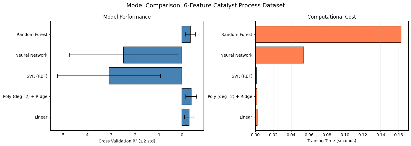
Let’s compare all nonlinear methods on a more challenging dataset with 6 features: the ensemble_process.csv dataset from a catalytic reactor simulation.

# Load 6-feature catalyst process dataset
url_proc = "https://raw.githubusercontent.com/jkitchin/s26-06642/main/dsmles/data/ensemble_process.csv"
df_proc = pd.read_csv(url_proc)

feature_cols = ["temperature", "pressure", "catalyst_loading",
                "residence_time", "feed_ratio", "impurity_level"]
X_proc = df_proc[feature_cols].values
y_proc = df_proc["conversion"].values

X_tr, X_te, y_tr, y_te = train_test_split(X_proc, y_proc, test_size=0.2, random_state=42)

print(f"Dataset: {X_proc.shape[0]} samples, {X_proc.shape[1]} features")
print(f"Target: reactor conversion")

Dataset: 500 samples, 6 features
Target: reactor conversion

# Compare five nonlinear approaches
models = {
    "Linear": Pipeline([
        ("scaler", StandardScaler()),
        ("model", LinearRegression())
    ]),
    "Poly (deg=2) + Ridge": Pipeline([
        ("scaler", StandardScaler()),
        ("poly", PolynomialFeatures(degree=2, include_bias=False)),
        ("model", Ridge(alpha=1.0))
    ]),
    "SVR (RBF)": Pipeline([
        ("scaler", StandardScaler()),
        ("model", SVR(kernel="rbf", C=100))
    ]),
    "Neural Network": Pipeline([
        ("scaler", StandardScaler()),
        ("model", MLPRegressor(hidden_layer_sizes=(100, 50), max_iter=1000, random_state=42))
    ]),
    "Random Forest": RandomForestRegressor(
        n_estimators=100, max_depth=10, random_state=42, n_jobs=-1
    ),
}

comparison = []
for name, model in models.items():
    start = time.time()
    model.fit(X_tr, y_tr)
    train_time = time.time() - start
    
    cv = RepeatedKFold(n_splits=5, n_repeats=2, random_state=42)
    cv_scores = cross_val_score(model, X_proc, y_proc, cv=cv, scoring="r2")
    
    comparison.append({
        "Model": name,
        "Train R²": model.score(X_tr, y_tr),
        "Test R²": model.score(X_te, y_te),
        "CV R² (mean)": cv_scores.mean(),
        "CV R² (std)": cv_scores.std(),
        "Train Time (s)": train_time
    })

comp_df = pd.DataFrame(comparison)
print(comp_df.to_string(index=False))

               Model  Train R²   Test R²  CV R² (mean)  CV R² (std)  Train Time (s)
              Linear  0.384361  0.086325      0.303848     0.098320        0.002024
Poly (deg=2) + Ridge  0.536004  0.164005      0.387165     0.112790        0.001715
           SVR (RBF) -3.016716 -3.880723     -3.038570     1.073372        0.001154
      Neural Network -0.586620 -2.355595     -2.426512     1.128295        0.053883
       Random Forest  0.899076  0.173614      0.358761     0.104775        0.162799

# Visualize model comparison
fig, axes = plt.subplots(1, 2, figsize=(14, 5))

# Left: CV R² with error bars
axes[0].barh(comp_df["Model"], comp_df["CV R² (mean)"],
             xerr=comp_df["CV R² (std)"] * 2, capsize=5,
             edgecolor="black", color="steelblue")
axes[0].set_xlabel("Cross-Validation R² (±2 std)")
axes[0].set_title("Model Performance")
axes[0].grid(True, alpha=0.3, axis="x")

# Right: Training time
axes[1].barh(comp_df["Model"], comp_df["Train Time (s)"],
             edgecolor="black", color="coral")
axes[1].set_xlabel("Training Time (seconds)")
axes[1].set_title("Computational Cost")
axes[1].grid(True, alpha=0.3, axis="x")

plt.suptitle("Model Comparison: 6-Feature Catalyst Process Dataset", fontsize=14)
plt.tight_layout()
plt.show()

../_images/114fb63cabe0d0addcd038feaed02a469781e00f95927e57e68c7d8128919107.png

When to Use Which Method#

Method	Scaling Needed?	Interpretable?	Tuning Difficulty	Best For
Linear/Ridge	Yes	High	Low	Baseline, few features
Polynomial + Ridge	Yes	Medium	Low-Medium	Known polynomial form, few features
SVR (RBF)	Yes	Low	Medium	Unknown nonlinearity, small datasets
Neural Network	Yes	Low	High	Complex patterns, enough data
Random Forest	No	Medium	Low	Good default, handles interactions

Practical advice: Start with Random Forest as a quick baseline (minimal tuning needed), then try neural networks or SVR if you need better performance and have time to tune.

%pip install -q jupyterquiz
from jupyterquiz import display_quiz

display_quiz("quizzes/neural-networks-hyperparameter-tuning-quiz.json")

Note: you may need to restart the kernel to use updated packages.

Summary#

What We Learned#

Topic	Key Takeaway
MLPRegressor	Universal approximator — flexible but needs careful tuning
Hidden layers	More neurons = more capacity, but risk of overfitting
Feature scaling	Essential for NNs and SVR; not needed for Random Forest
Alpha	L2 regularization — same concept as Ridge, applied to network weights
Random Forest	Strong baseline with minimal tuning; covered in depth in Module 10
RandomizedSearchCV	Efficient alternative to grid search for large parameter spaces
RepeatedKFold	More stable CV estimates through repeated splitting

The Tuning Lesson#

A well-tuned simple model often beats a poorly tuned complex model. The algorithm isn’t magic — systematic tuning is essential. This is especially true for neural networks, which have many interacting hyperparameters.

Common Pitfalls#

Forgetting to scale features for neural networks (use Pipeline!)
Using default hyperparameters and expecting good results
Exhaustive grid search when random search would be faster and equally effective
Trusting a single train/test split instead of cross-validation
Choosing the most complex model when a simpler one performs comparably

Next Steps#

Module 10 covers ensemble methods in depth — Random Forests, Gradient Boosting, and XGBoost. These combine multiple models for even better predictions, and they’ll prove crucial in the ongoing catalyst investigation.

The Catalyst Crisis: Chapter 9b - “The Humbling”#

A story about the gap between promise and practice

Maya was excited. “Neural networks. Universal approximators. They can learn any function.”

She’d read three papers that morning and was ready to solve the catalyst mystery once and for all. She opened a notebook, imported MLPRegressor, and fed it the reactor data.

The first result: R-squared of 0.12.

“That can’t be right.” She re-ran it. Same result. She added more neurons. 0.15. She added more layers. 0.08. She doubled everything. 0.03.

“It’s getting worse?”

Alex looked over her shoulder. “Did you scale the features?”

Maya checked. Temperature was in the hundreds, pressure in the tens, impurity levels in the hundredths. The network was drowning in scale differences.

She added StandardScaler in a pipeline. R-squared jumped to 0.45. Better, but not the breakthrough she’d hoped for.

“Try different architectures,” Sam suggested. “And different learning rates. And alpha values.”

Three hours later, Maya had a spreadsheet of 47 experiments. Some configurations scored 0.50. Others scored 0.10. One bizarre combination of tanh activation with a tiny learning rate scored 0.55. Nothing was consistent.

“I thought neural networks were supposed to be powerful,” she said, frustration creeping in.

“They are,” Alex said. “But power without tuning is just chaos. A badly tuned neural network is worse than a simple linear model.”

Professor Pipeline, passing through the lab, overheard. “What have you tried?”

“Everything.” Maya gestured at the spreadsheet.

“No. You’ve tried random things. That’s not the same as everything.” He sat down. “You need RandomizedSearchCV. Define the space, set a budget, let the search be systematic. And use RepeatedKFold so your scores are stable.”

Maya refactored her code. The randomized search ran thirty configurations in minutes. The best scored 0.52, repeatable across folds. Not spectacular, but honest.

“The algorithm isn’t magic,” Alex said. “It’s a tool. And tools need to be calibrated.”

Maya nodded slowly. She’d been humbled—not by the problem, but by her own assumptions. The neural network could learn anything in theory. In practice, it needed help: the right scale, the right architecture, the right regularization. Systematic tuning, not hopeful guessing.

“You know what worked almost as well with zero tuning?” Sam showed her a Random Forest result. R-squared of 0.48, out of the box.

Maya laughed. “So the fancy model barely beats the simple one?”

“For now,” Professor Pipeline said. “But the ensemble methods in our next lesson—when you combine many models together—that’s when things get interesting. That’s when patterns emerge that no single model can find alone.”

He left. Maya stared at her results. The catalyst mystery wasn’t solved. But she’d learned something that might matter more: the gap between a model’s theoretical power and its practical performance is bridged by careful, systematic tuning.

She added to the mystery board: Tuning matters more than algorithm choice. Next: ensemble methods.

Continue to Module 10 to discover the power of ensemble methods…

	steps steps: list of tuples List of (name of step, estimator) tuples that are to be chained in sequential order. To be compatible with the scikit-learn API, all steps must define `fit`. All non-last steps must also define `transform`. See :ref:`Combining Estimators ` for more details.	[('scaler', ...), ('mlp', ...)]
	transform_input transform_input: list of str, default=None The names of the :term:`metadata` parameters that should be transformed by the pipeline before passing it to the step consuming it. This enables transforming some input arguments to ``fit`` (other than ``X``) to be transformed by the steps of the pipeline up to the step which requires them. Requirement is defined via :ref:`metadata routing `. For instance, this can be used to pass a validation set through the pipeline. You can only set this if metadata routing is enabled, which you can enable using ``sklearn.set_config(enable_metadata_routing=True)``. .. versionadded:: 1.6	None
	memory memory: str or object with the joblib.Memory interface, default=None Used to cache the fitted transformers of the pipeline. The last step will never be cached, even if it is a transformer. By default, no caching is performed. If a string is given, it is the path to the caching directory. Enabling caching triggers a clone of the transformers before fitting. Therefore, the transformer instance given to the pipeline cannot be inspected directly. Use the attribute ``named_steps`` or ``steps`` to inspect estimators within the pipeline. Caching the transformers is advantageous when fitting is time consuming. See :ref:`sphx_glr_auto_examples_neighbors_plot_caching_nearest_neighbors.py` for an example on how to enable caching.	None
	verbose verbose: bool, default=False If True, the time elapsed while fitting each step will be printed as it is completed.	False

	loss loss: {'squared_error', 'poisson'}, default='squared_error' The loss function to use when training the weights. Note that the "squared error" and "poisson" losses actually implement "half squares error" and "half poisson deviance" to simplify the computation of the gradient. Furthermore, the "poisson" loss internally uses a log-link (exponential as the output activation function) and requires ``y >= 0``. .. versionchanged:: 1.7 Added parameter `loss` and option 'poisson'.	'squared_error'
	hidden_layer_sizes hidden_layer_sizes: array-like of shape(n_layers - 2,), default=(100,) The ith element represents the number of neurons in the ith hidden layer.	(100,)
	activation activation: {'identity', 'logistic', 'tanh', 'relu'}, default='relu' Activation function for the hidden layer. - 'identity', no-op activation, useful to implement linear bottleneck, returns f(x) = x - 'logistic', the logistic sigmoid function, returns f(x) = 1 / (1 + exp(-x)). - 'tanh', the hyperbolic tan function, returns f(x) = tanh(x). - 'relu', the rectified linear unit function, returns f(x) = max(0, x)	'tanh'
	solver solver: {'lbfgs', 'sgd', 'adam'}, default='adam' The solver for weight optimization. - 'lbfgs' is an optimizer in the family of quasi-Newton methods. - 'sgd' refers to stochastic gradient descent. - 'adam' refers to a stochastic gradient-based optimizer proposed by Kingma, Diederik, and Jimmy Ba For a comparison between Adam optimizer and SGD, see :ref:`sphx_glr_auto_examples_neural_networks_plot_mlp_training_curves.py`. Note: The default solver 'adam' works pretty well on relatively large datasets (with thousands of training samples or more) in terms of both training time and validation score. For small datasets, however, 'lbfgs' can converge faster and perform better.	'lbfgs'
	alpha alpha: float, default=0.0001 Strength of the L2 regularization term. The L2 regularization term is divided by the sample size when added to the loss.	0.0001
	batch_size batch_size: int, default='auto' Size of minibatches for stochastic optimizers. If the solver is 'lbfgs', the regressor will not use minibatch. When set to "auto", `batch_size=min(200, n_samples)`.	'auto'
	learning_rate learning_rate: {'constant', 'invscaling', 'adaptive'}, default='constant' Learning rate schedule for weight updates. - 'constant' is a constant learning rate given by 'learning_rate_init'. - 'invscaling' gradually decreases the learning rate ``learning_rate_`` at each time step 't' using an inverse scaling exponent of 'power_t'. effective_learning_rate = learning_rate_init / pow(t, power_t) - 'adaptive' keeps the learning rate constant to 'learning_rate_init' as long as training loss keeps decreasing. Each time two consecutive epochs fail to decrease training loss by at least tol, or fail to increase validation score by at least tol if 'early_stopping' is on, the current learning rate is divided by 5. Only used when solver='sgd'.	'constant'
	learning_rate_init learning_rate_init: float, default=0.001 The initial learning rate used. It controls the step-size in updating the weights. Only used when solver='sgd' or 'adam'.	0.001
	power_t power_t: float, default=0.5 The exponent for inverse scaling learning rate. It is used in updating effective learning rate when the learning_rate is set to 'invscaling'. Only used when solver='sgd'.	0.5
	max_iter max_iter: int, default=200 Maximum number of iterations. The solver iterates until convergence (determined by 'tol') or this number of iterations. For stochastic solvers ('sgd', 'adam'), note that this determines the number of epochs (how many times each data point will be used), not the number of gradient steps.	1000
	shuffle shuffle: bool, default=True Whether to shuffle samples in each iteration. Only used when solver='sgd' or 'adam'.	True
	random_state random_state: int, RandomState instance, default=None Determines random number generation for weights and bias initialization, train-test split if early stopping is used, and batch sampling when solver='sgd' or 'adam'. Pass an int for reproducible results across multiple function calls. See :term:`Glossary `.	42
	tol tol: float, default=1e-4 Tolerance for the optimization. When the loss or score is not improving by at least ``tol`` for ``n_iter_no_change`` consecutive iterations, unless ``learning_rate`` is set to 'adaptive', convergence is considered to be reached and training stops.	0.0001
	verbose verbose: bool, default=False Whether to print progress messages to stdout.	False
	warm_start warm_start: bool, default=False When set to True, reuse the solution of the previous call to fit as initialization, otherwise, just erase the previous solution. See :term:`the Glossary `.	False
	momentum momentum: float, default=0.9 Momentum for gradient descent update. Should be between 0 and 1. Only used when solver='sgd'.	0.9
	nesterovs_momentum nesterovs_momentum: bool, default=True Whether to use Nesterov's momentum. Only used when solver='sgd' and momentum > 0.	True
	early_stopping early_stopping: bool, default=False Whether to use early stopping to terminate training when validation score is not improving. If set to True, it will automatically set aside ``validation_fraction`` of training data as validation and terminate training when validation score is not improving by at least ``tol`` for ``n_iter_no_change`` consecutive epochs. Only effective when solver='sgd' or 'adam'.	False
	validation_fraction validation_fraction: float, default=0.1 The proportion of training data to set aside as validation set for early stopping. Must be between 0 and 1. Only used if early_stopping is True.	0.1
	beta_1 beta_1: float, default=0.9 Exponential decay rate for estimates of first moment vector in adam, should be in [0, 1). Only used when solver='adam'.	0.9
	beta_2 beta_2: float, default=0.999 Exponential decay rate for estimates of second moment vector in adam, should be in [0, 1). Only used when solver='adam'.	0.999
	epsilon epsilon: float, default=1e-8 Value for numerical stability in adam. Only used when solver='adam'.	1e-08
	n_iter_no_change n_iter_no_change: int, default=10 Maximum number of epochs to not meet ``tol`` improvement. Only effective when solver='sgd' or 'adam'. .. versionadded:: 0.20	10
	max_fun max_fun: int, default=15000 Only used when solver='lbfgs'. Maximum number of function calls. The solver iterates until convergence (determined by ``tol``), number of iterations reaches max_iter, or this number of function calls. Note that number of function calls will be greater than or equal to the number of iterations for the MLPRegressor. .. versionadded:: 0.22	15000

	n_estimators n_estimators: int, default=100 The number of trees in the forest. .. versionchanged:: 0.22 The default value of ``n_estimators`` changed from 10 to 100 in 0.22.	100
	criterion criterion: {"squared_error", "absolute_error", "friedman_mse", "poisson"}, default="squared_error" The function to measure the quality of a split. Supported criteria are "squared_error" for the mean squared error, which is equal to variance reduction as feature selection criterion and minimizes the L2 loss using the mean of each terminal node, "friedman_mse", which uses mean squared error with Friedman's improvement score for potential splits, "absolute_error" for the mean absolute error, which minimizes the L1 loss using the median of each terminal node, and "poisson" which uses reduction in Poisson deviance to find splits. Training using "absolute_error" is significantly slower than when using "squared_error". .. versionadded:: 0.18 Mean Absolute Error (MAE) criterion. .. versionadded:: 1.0 Poisson criterion.	'squared_error'
	max_depth max_depth: int, default=None The maximum depth of the tree. If None, then nodes are expanded until all leaves are pure or until all leaves contain less than min_samples_split samples.	10
	min_samples_split min_samples_split: int or float, default=2 The minimum number of samples required to split an internal node: - If int, then consider `min_samples_split` as the minimum number. - If float, then `min_samples_split` is a fraction and `ceil(min_samples_split * n_samples)` are the minimum number of samples for each split. .. versionchanged:: 0.18 Added float values for fractions.	2
	min_samples_leaf min_samples_leaf: int or float, default=1 The minimum number of samples required to be at a leaf node. A split point at any depth will only be considered if it leaves at least ``min_samples_leaf`` training samples in each of the left and right branches. This may have the effect of smoothing the model, especially in regression. - If int, then consider `min_samples_leaf` as the minimum number. - If float, then `min_samples_leaf` is a fraction and `ceil(min_samples_leaf * n_samples)` are the minimum number of samples for each node. .. versionchanged:: 0.18 Added float values for fractions.	1
	min_weight_fraction_leaf min_weight_fraction_leaf: float, default=0.0 The minimum weighted fraction of the sum total of weights (of all the input samples) required to be at a leaf node. Samples have equal weight when sample_weight is not provided.	0.0
	max_features max_features: {"sqrt", "log2", None}, int or float, default=1.0 The number of features to consider when looking for the best split: - If int, then consider `max_features` features at each split. - If float, then `max_features` is a fraction and `max(1, int(max_features * n_features_in_))` features are considered at each split. - If "sqrt", then `max_features=sqrt(n_features)`. - If "log2", then `max_features=log2(n_features)`. - If None or 1.0, then `max_features=n_features`. .. note:: The default of 1.0 is equivalent to bagged trees and more randomness can be achieved by setting smaller values, e.g. 0.3. .. versionchanged:: 1.1 The default of `max_features` changed from `"auto"` to 1.0. Note: the search for a split does not stop until at least one valid partition of the node samples is found, even if it requires to effectively inspect more than ``max_features`` features.	1.0
	max_leaf_nodes max_leaf_nodes: int, default=None Grow trees with ``max_leaf_nodes`` in best-first fashion. Best nodes are defined as relative reduction in impurity. If None then unlimited number of leaf nodes.	None
	min_impurity_decrease min_impurity_decrease: float, default=0.0 A node will be split if this split induces a decrease of the impurity greater than or equal to this value. The weighted impurity decrease equation is the following:: N_t / N * (impurity - N_t_R / N_t * right_impurity - N_t_L / N_t * left_impurity) where ``N`` is the total number of samples, ``N_t`` is the number of samples at the current node, ``N_t_L`` is the number of samples in the left child, and ``N_t_R`` is the number of samples in the right child. ``N``, ``N_t``, ``N_t_R`` and ``N_t_L`` all refer to the weighted sum, if ``sample_weight`` is passed. .. versionadded:: 0.19	0.0
	bootstrap bootstrap: bool, default=True Whether bootstrap samples are used when building trees. If False, the whole dataset is used to build each tree.	True
	oob_score oob_score: bool or callable, default=False Whether to use out-of-bag samples to estimate the generalization score. By default, :func:`~sklearn.metrics.r2_score` is used. Provide a callable with signature `metric(y_true, y_pred)` to use a custom metric. Only available if `bootstrap=True`. For an illustration of out-of-bag (OOB) error estimation, see the example :ref:`sphx_glr_auto_examples_ensemble_plot_ensemble_oob.py`.	False
	n_jobs n_jobs: int, default=None The number of jobs to run in parallel. :meth:`fit`, :meth:`predict`, :meth:`decision_path` and :meth:`apply` are all parallelized over the trees. ``None`` means 1 unless in a :obj:`joblib.parallel_backend` context. ``-1`` means using all processors. See :term:`Glossary ` for more details.	-1
	random_state random_state: int, RandomState instance or None, default=None Controls both the randomness of the bootstrapping of the samples used when building trees (if ``bootstrap=True``) and the sampling of the features to consider when looking for the best split at each node (if ``max_features < n_features``). See :term:`Glossary ` for details.	42
	verbose verbose: int, default=0 Controls the verbosity when fitting and predicting.	0
	warm_start warm_start: bool, default=False When set to ``True``, reuse the solution of the previous call to fit and add more estimators to the ensemble, otherwise, just fit a whole new forest. See :term:`Glossary ` and :ref:`tree_ensemble_warm_start` for details.	False
	ccp_alpha ccp_alpha: non-negative float, default=0.0 Complexity parameter used for Minimal Cost-Complexity Pruning. The subtree with the largest cost complexity that is smaller than ``ccp_alpha`` will be chosen. By default, no pruning is performed. See :ref:`minimal_cost_complexity_pruning` for details. See :ref:`sphx_glr_auto_examples_tree_plot_cost_complexity_pruning.py` for an example of such pruning. .. versionadded:: 0.22	0.0
	max_samples max_samples: int or float, default=None If bootstrap is True, the number of samples to draw from X to train each base estimator. - If None (default), then draw `X.shape[0]` samples. - If int, then draw `max_samples` samples. - If float, then draw `max(round(n_samples * max_samples), 1)` samples. Thus, `max_samples` should be in the interval `(0.0, 1.0]`. .. versionadded:: 0.22	None
	monotonic_cst monotonic_cst: array-like of int of shape (n_features), default=None Indicates the monotonicity constraint to enforce on each feature. - 1: monotonically increasing - 0: no constraint - -1: monotonically decreasing If monotonic_cst is None, no constraints are applied. Monotonicity constraints are not supported for: - multioutput regressions (i.e. when `n_outputs_ > 1`), - regressions trained on data with missing values. Read more in the :ref:`User Guide `. .. versionadded:: 1.4	None

Neural Networks and Hyperparameter Tuning

Contents

Neural Networks and Hyperparameter Tuning#

Learning Objectives#

Neural Networks with sklearn#

Why Neural Networks?#

How MLPRegressor Works#

Key Hyperparameters#

Effect of Hidden Layer Size#

Activation Functions#

Feature Scaling is Essential#

Alpha: L2 Regularization#

Solver Choice#

Early Stopping#

Random Forest Preview#

From Trees to Forests#

Key Hyperparameters#

No Scaling Required#

Hyperparameter Tuning Strategies#

The Challenge#

GridSearchCV Review#

RandomizedSearchCV: A Smarter Approach#

Choosing Distributions#

Cross-Validation Strategies#

RepeatedKFold#

Model Comparison on a Higher-Dimensional Problem#

When to Use Which Method#

Recommended Reading#

Summary#

What We Learned#

The Tuning Lesson#

Common Pitfalls#

Next Steps#

The Catalyst Crisis: Chapter 9b - “The Humbling”#

	copy copy: bool, default=True If False, try to avoid a copy and do inplace scaling instead. This is not guaranteed to always work inplace; e.g. if the data is not a NumPy array or scipy.sparse CSR matrix, a copy may still be returned.	True
	with_mean with_mean: bool, default=True If True, center the data before scaling. This does not work (and will raise an exception) when attempted on sparse matrices, because centering them entails building a dense matrix which in common use cases is likely to be too large to fit in memory.	True
	with_std with_std: bool, default=True If True, scale the data to unit variance (or equivalently, unit standard deviation).	True