Module 08: Regularization and Model Selection

Preventing overfitting and choosing the best model.

Learning Objectives

1. Understand overfitting and the bias-variance tradeoff

2. Apply Ridge, Lasso, and ElasticNet regularization

3. Use cross-validation for model selection

4. Tune hyperparameters systematically

5. Compare models fairly

import numpy as np
import pandas as pd
import matplotlib.pyplot as plt
from sklearn.linear_model import LinearRegression, Ridge, Lasso, ElasticNet
from sklearn.linear_model import RidgeCV, LassoCV, ElasticNetCV
from sklearn.model_selection import train_test_split, cross_val_score, KFold
from sklearn.preprocessing import StandardScaler, PolynomialFeatures
from sklearn.metrics import mean_squared_error, r2_score
from sklearn.pipeline import Pipeline

The Overfitting Problem: Why Complex Models Fail

Overfitting is the central challenge in machine learning. Understanding it is crucial.

What Is Overfitting?

A model that memorizes the training data instead of learning generalizable patterns. It fits the noise, not the signal.

The Bias-Variance Tradeoff

Every model makes two types of errors:

Bias (underfitting): Error from oversimplifying. A linear model can’t capture nonlinear relationships, no matter how much data you have.

Variance (overfitting): Error from being too sensitive to training data. A very flexible model will fit different training sets very differently.

Model Complexity	Bias	Variance	Result
Too simple	High	Low	Underfitting: misses patterns
Just right	Medium	Medium	Generalizes well
Too complex	Low	High	Overfitting: memorizes noise

When Overfitting Happens

You’re at risk when:

• Many features, few samples: More parameters than data points to constrain them

• Features are correlated: Multiple ways to explain the same variance

• Model is very flexible: High-degree polynomials, deep trees, etc.

• No regularization: Nothing preventing the model from fitting noise

# Load sparse regression dataset
import pandas as pd
import numpy as np
from sklearn.model_selection import train_test_split

url = "https://raw.githubusercontent.com/jkitchin/s26-06642/main/dsmles/data/sparse_regression.csv"
df = pd.read_csv(url)

# Extract features and target
feature_cols = [col for col in df.columns if col != 'target']
X = df[feature_cols].values
n_features = X.shape[1]
y = df['target'].values

# Load true coefficients for reference
url_coef = "https://raw.githubusercontent.com/jkitchin/s26-06642/main/dsmles/data/sparse_regression_true_coef.csv"
true_coef_df = pd.read_csv(url_coef)
true_coef = true_coef_df['true_coef'].values

# Split data
X_train, X_test, y_train, y_test = train_test_split(X, y, test_size=0.3, random_state=42)

print(f"Dataset: {X.shape[0]} samples, {X.shape[1]} features")
print(f"Training: {X_train.shape[0]} samples, Test: {X_test.shape[0]} samples")
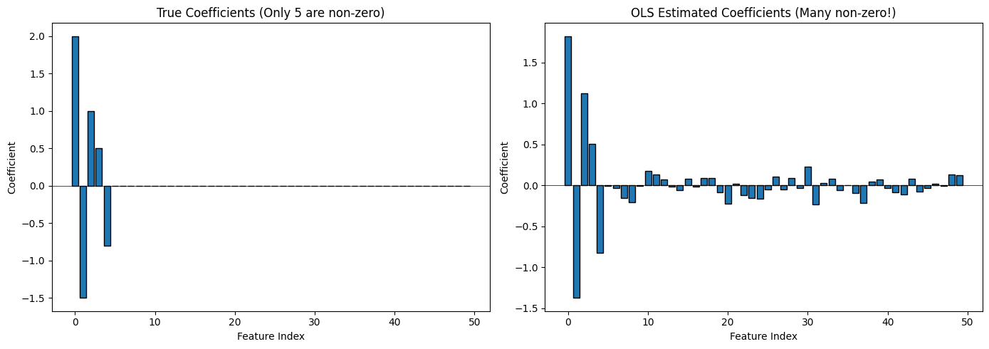
print(f"True non-zero coefficients at indices: {np.where(true_coef != 0)[0]}")

Dataset: 100 samples, 50 features
Training: 70 samples, Test: 30 samples
True non-zero coefficients at indices: [0 1 2 3 4]

# Ordinary Least Squares (OLS) - no regularization
ols = LinearRegression()
ols.fit(X_train, y_train)

print("OLS (No Regularization):")
print(f"  Training R²: {ols.score(X_train, y_train):.4f}")
print(f"  Test R²: {ols.score(X_test, y_test):.4f}")
print(f"  Gap: {ols.score(X_train, y_train) - ols.score(X_test, y_test):.4f}")

OLS (No Regularization):
  Training R²: 0.9927
  Test R²: 0.8884
  Gap: 0.1043

# Compare OLS coefficients to true coefficients
fig, axes = plt.subplots(1, 2, figsize=(14, 5))

# True coefficients
axes[0].bar(range(n_features), true_coef, edgecolor='black')
axes[0].set_xlabel('Feature Index')
axes[0].set_ylabel('Coefficient')
axes[0].set_title('True Coefficients (Only 5 are non-zero)')
axes[0].axhline(y=0, color='black', linestyle='-', linewidth=0.5)

# OLS coefficients
axes[1].bar(range(n_features), ols.coef_, edgecolor='black')
axes[1].set_xlabel('Feature Index')
axes[1].set_ylabel('Coefficient')
axes[1].set_title('OLS Estimated Coefficients (Many non-zero!)')
axes[1].axhline(y=0, color='black', linestyle='-', linewidth=0.5)

plt.tight_layout()
plt.show()

Ridge Regression (L2 Regularization): Shrink, Don’t Select

Ridge regression adds a penalty on the sum of squared coefficients:

\[\min_\beta \|y - X\beta\|^2 + \alpha \|\beta\|^2\]

The Key Insight

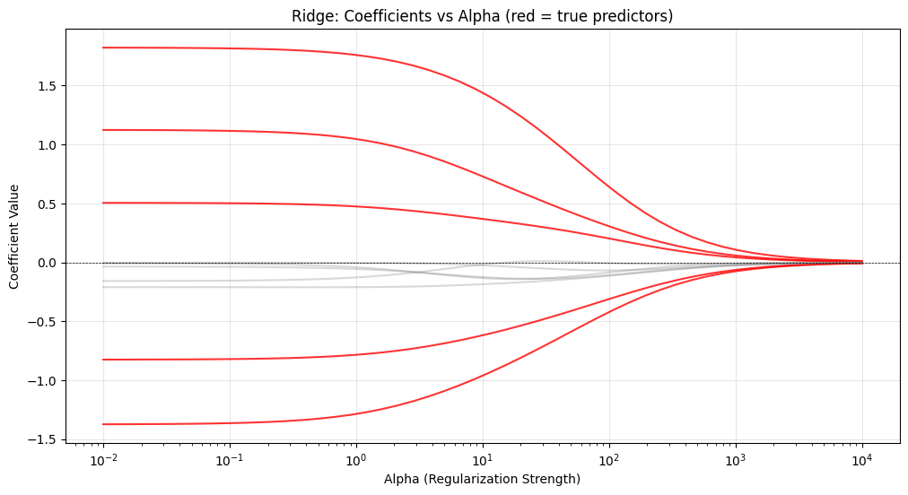
Ridge shrinks coefficients toward zero but never exactly to zero. All features stay in the model, just with smaller effects.

When to Use Ridge

• Multicollinearity: Correlated features cause unstable OLS coefficients. Ridge stabilizes them.

• Many features: Even if all features might be relevant, you want smaller, more stable coefficients.

• Prediction focus: You care more about prediction accuracy than identifying which features matter.

The Alpha Parameter

• α = 0: Pure OLS, no regularization

• α → ∞: All coefficients shrink to zero

• Optimal α: Found via cross-validation

# Ridge regression
ridge = Ridge(alpha=1.0)
ridge.fit(X_train, y_train)

print("Ridge Regression (alpha=1.0):")
print(f"  Training R²: {ridge.score(X_train, y_train):.4f}")
print(f"  Test R²: {ridge.score(X_test, y_test):.4f}")
print(f"  Gap: {ridge.score(X_train, y_train) - ridge.score(X_test, y_test):.4f}")

Ridge Regression (alpha=1.0):
  Training R²: 0.9920
  Test R²: 0.8792
  Gap: 0.1128

# Effect of alpha on coefficients
alphas = np.logspace(-2, 4, 50)
ridge_coefs = []

for alpha in alphas:
    ridge = Ridge(alpha=alpha)
    ridge.fit(X_train, y_train)
    ridge_coefs.append(ridge.coef_)

ridge_coefs = np.array(ridge_coefs)

plt.figure(figsize=(12, 6))
for i in range(10):  # Plot first 10 features
    color = 'red' if i < 5 else 'gray'  # Red for true predictors
    alpha_val = 0.8 if i < 5 else 0.3
    plt.semilogx(alphas, ridge_coefs[:, i], color=color, alpha=alpha_val)

plt.xlabel('Alpha (Regularization Strength)')
plt.ylabel('Coefficient Value')
plt.title('Ridge: Coefficients vs Alpha (red = true predictors)')
plt.axhline(y=0, color='black', linestyle='--', linewidth=0.5)
plt.grid(True, alpha=0.3)
plt.show()

Lasso Regression (L1 Regularization): Shrink AND Select

Lasso adds a penalty on the sum of absolute coefficients:

\[\min_\beta \|y - X\beta\|^2 + \alpha \|\beta\|_1\]

The Key Insight

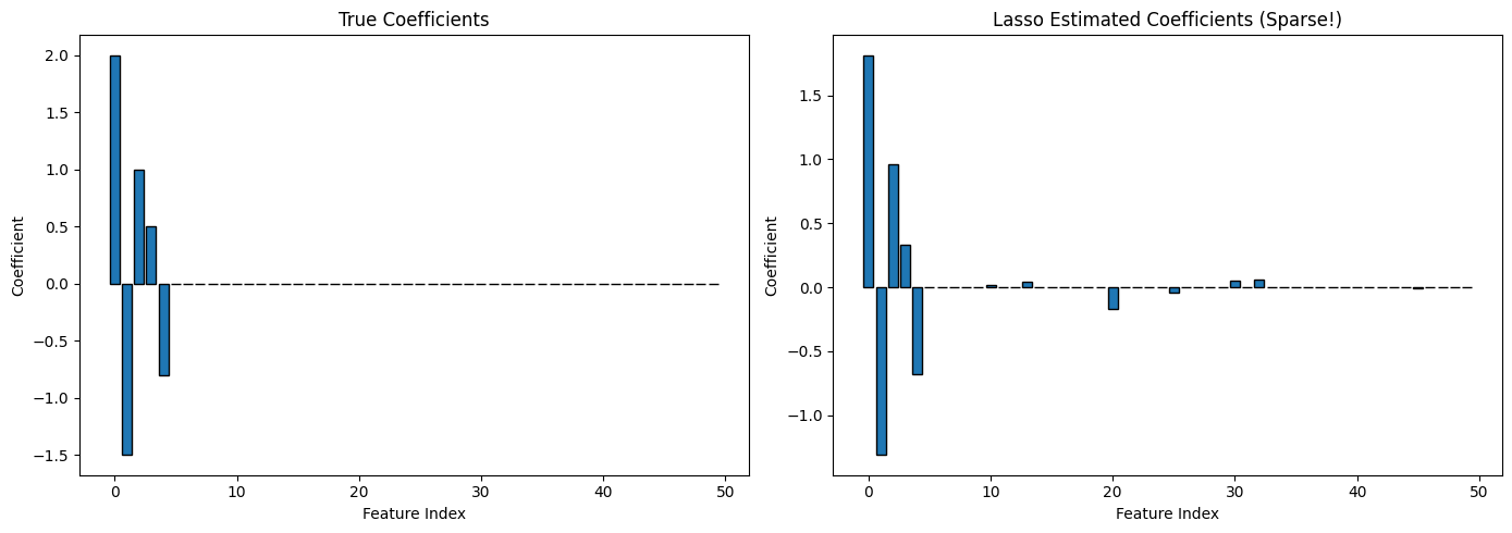
The L1 penalty has a remarkable property: it drives some coefficients exactly to zero. Lasso performs automatic feature selection!

Why L1 Creates Sparsity (Intuition)

Imagine you’re trying to reduce the total “cost” of coefficients. With L2 (squared), reducing a large coefficient saves more than eliminating a small one. With L1 (absolute), eliminating a coefficient entirely saves just as much per unit as shrinking a large one. The optimizer often chooses to eliminate.

When to Use Lasso

• Feature selection needed: You suspect many features are irrelevant

• Interpretability: You want a sparse model with only important features

• High dimensionality: When p > n (more features than samples)

The Tradeoff

Lasso can be unstable with correlated features—it might arbitrarily pick one and zero out the others. If you need stable selection of correlated features, consider ElasticNet.

# Lasso regression
lasso = Lasso(alpha=0.1, max_iter=10000)
lasso.fit(X_train, y_train)

print("Lasso Regression (alpha=0.1):")
print(f"  Training R²: {lasso.score(X_train, y_train):.4f}")
print(f"  Test R²: {lasso.score(X_test, y_test):.4f}")
print(f"  Non-zero coefficients: {np.sum(lasso.coef_ != 0)} out of {n_features}")

Lasso Regression (alpha=0.1):
  Training R²: 0.9677
  Test R²: 0.9578
  Non-zero coefficients: 13 out of 50

# Compare Lasso to true coefficients
fig, axes = plt.subplots(1, 2, figsize=(14, 5))

# True coefficients
axes[0].bar(range(n_features), true_coef, edgecolor='black')
axes[0].set_xlabel('Feature Index')
axes[0].set_ylabel('Coefficient')
axes[0].set_title('True Coefficients')

# Lasso coefficients
axes[1].bar(range(n_features), lasso.coef_, edgecolor='black')
axes[1].set_xlabel('Feature Index')
axes[1].set_ylabel('Coefficient')
axes[1].set_title('Lasso Estimated Coefficients (Sparse!)')

plt.tight_layout()
plt.show()

ElasticNet (Combined L1 + L2)

ElasticNet combines both penalties:

\[\min_\beta \|y - X\beta\|^2 + \alpha \cdot l1\_ratio \cdot \|\beta\|_1 + \alpha \cdot (1 - l1\_ratio) \cdot \|\beta\|^2\]

• l1_ratio=1: Pure Lasso

• l1_ratio=0: Pure Ridge

• l1_ratio=0.5: Balanced mix

# ElasticNet
elastic = ElasticNet(alpha=0.1, l1_ratio=0.5, max_iter=10000)
elastic.fit(X_train, y_train)

print("ElasticNet (alpha=0.1, l1_ratio=0.5):")
print(f"  Training R²: {elastic.score(X_train, y_train):.4f}")
print(f"  Test R²: {elastic.score(X_test, y_test):.4f}")
print(f"  Non-zero coefficients: {np.sum(elastic.coef_ != 0)}")

ElasticNet (alpha=0.1, l1_ratio=0.5):
  Training R²: 0.9739
  Test R²: 0.9302
  Non-zero coefficients: 27

Cross-Validation: The Right Way to Evaluate Models

A single train/test split is noisy. The test performance depends on which points happened to be in the test set. Cross-validation gives more reliable estimates.

How K-Fold Cross-Validation Works

1. Split data into k equal parts (folds)

2. For each fold:

   • Train on k-1 folds

   • Test on the remaining fold

3. Average the k test scores

Why It’s Better

• Uses all data for both training and testing

• Provides error bars (standard deviation across folds)

• Less sensitive to the random split

Choosing K

K	Pros	Cons
5	Fast, reasonable variance estimate	Some bias if dataset is small
10	Good balance, common default	Slower than 5-fold
n (Leave-One-Out)	Minimum bias	High variance, slow, rarely used

Rule of thumb: K=5 or K=10 works well for most problems.

# 5-fold cross-validation
from sklearn.model_selection import cross_val_score

# Use full dataset for CV
cv_scores_ols = cross_val_score(LinearRegression(), X, y, cv=5, scoring='r2')
cv_scores_ridge = cross_val_score(Ridge(alpha=1.0), X, y, cv=5, scoring='r2')
cv_scores_lasso = cross_val_score(Lasso(alpha=0.1, max_iter=10000), X, y, cv=5, scoring='r2')

print("5-Fold Cross-Validation R² Scores:")
print(f"  OLS:   {cv_scores_ols.mean():.4f} (+/- {cv_scores_ols.std()*2:.4f})")
print(f"  Ridge: {cv_scores_ridge.mean():.4f} (+/- {cv_scores_ridge.std()*2:.4f})")
print(f"  Lasso: {cv_scores_lasso.mean():.4f} (+/- {cv_scores_lasso.std()*2:.4f})")

5-Fold Cross-Validation R² Scores:
  OLS:   0.9282 (+/- 0.0707)
  Ridge: 0.9296 (+/- 0.0642)
  Lasso: 0.9462 (+/- 0.0471)

# Visualize CV process
kf = KFold(n_splits=5, shuffle=True, random_state=42)

fig, axes = plt.subplots(1, 5, figsize=(15, 2))

for i, (train_idx, test_idx) in enumerate(kf.split(X)):
    fold_array = np.zeros(len(X))
    fold_array[train_idx] = 1  # Training = 1
    fold_array[test_idx] = 2   # Test = 2
    
    axes[i].imshow([fold_array], aspect='auto', cmap='RdYlGn')
    axes[i].set_title(f'Fold {i+1}')
    axes[i].set_yticks([])
    axes[i].set_xlabel('Sample Index')

plt.suptitle('5-Fold Cross-Validation (Green=Train, Red=Test)')
plt.tight_layout()
plt.show()

Hyperparameter Tuning with CV

Use cross-validation to find the optimal regularization strength.

# RidgeCV: automatically finds best alpha
alphas = np.logspace(-4, 4, 50)

ridge_cv = RidgeCV(alphas=alphas, cv=5)
ridge_cv.fit(X_train, y_train)

print(f"Best Ridge alpha: {ridge_cv.alpha_:.4f}")
print(f"Test R²: {ridge_cv.score(X_test, y_test):.4f}")

Best Ridge alpha: 1.2068
Test R²: 0.8768

# LassoCV: automatically finds best alpha
lasso_cv = LassoCV(alphas=np.logspace(-4, 1, 50), cv=5, max_iter=10000)
lasso_cv.fit(X_train, y_train)

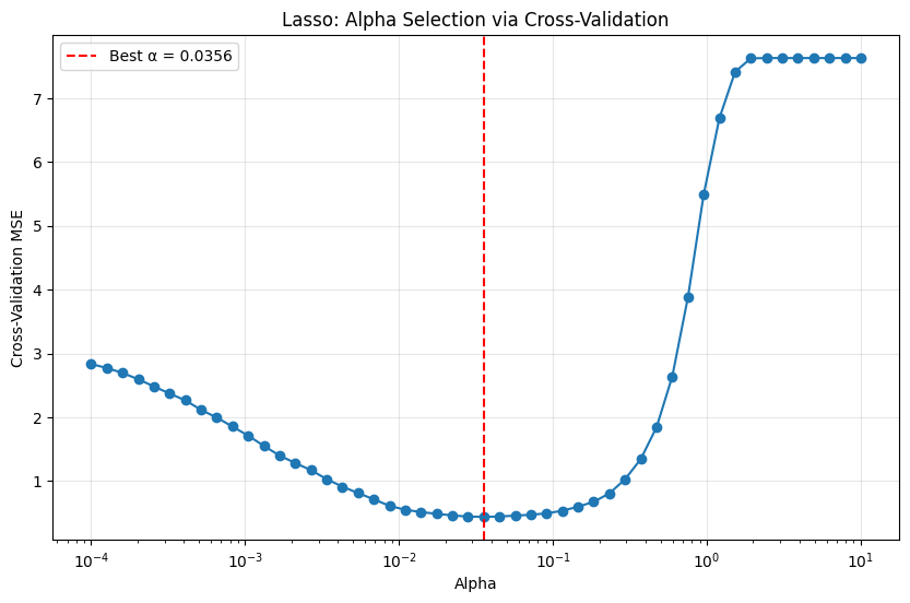
print(f"Best Lasso alpha: {lasso_cv.alpha_:.4f}")
print(f"Test R²: {lasso_cv.score(X_test, y_test):.4f}")
print(f"Non-zero coefficients: {np.sum(lasso_cv.coef_ != 0)}")

Best Lasso alpha: 0.0356
Test R²: 0.9660
Non-zero coefficients: 31

# Visualize alpha selection for Lasso
alphas_lasso = np.logspace(-4, 1, 50)
mse_path = []

for alpha in alphas_lasso:
    lasso = Lasso(alpha=alpha, max_iter=10000)
    scores = -cross_val_score(lasso, X_train, y_train, cv=5, scoring='neg_mean_squared_error')
    mse_path.append(scores.mean())

plt.figure(figsize=(10, 6))
plt.semilogx(alphas_lasso, mse_path, 'o-')
plt.axvline(x=lasso_cv.alpha_, color='r', linestyle='--', label=f'Best α = {lasso_cv.alpha_:.4f}')
plt.xlabel('Alpha')
plt.ylabel('Cross-Validation MSE')
plt.title('Lasso: Alpha Selection via Cross-Validation')
plt.legend()
plt.grid(True, alpha=0.3)
plt.show()

Grid Search for Multiple Hyperparameters

When you have multiple hyperparameters, use GridSearchCV.

from sklearn.model_selection import GridSearchCV

# Grid search for ElasticNet
param_grid = {
    'alpha': [0.001, 0.01, 0.1, 1.0],
    'l1_ratio': [0.1, 0.3, 0.5, 0.7, 0.9]
}

elastic = ElasticNet(max_iter=10000)
grid_search = GridSearchCV(elastic, param_grid, cv=5, scoring='r2')
grid_search.fit(X_train, y_train)

print(f"Best parameters: {grid_search.best_params_}")
print(f"Best CV score: {grid_search.best_score_:.4f}")
print(f"Test score: {grid_search.score(X_test, y_test):.4f}")

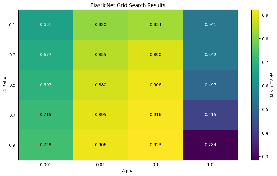
Best parameters: {'alpha': 0.1, 'l1_ratio': 0.9}
Best CV score: 0.9227
Test score: 0.9550

# Visualize grid search results
results = pd.DataFrame(grid_search.cv_results_)
pivot = results.pivot_table(
    values='mean_test_score',
    index='param_l1_ratio',
    columns='param_alpha'
)

plt.figure(figsize=(10, 6))
plt.imshow(pivot.values, cmap='viridis', aspect='auto')
plt.colorbar(label='Mean CV R²')
plt.xticks(range(len(pivot.columns)), pivot.columns)
plt.yticks(range(len(pivot.index)), pivot.index)
plt.xlabel('Alpha')
plt.ylabel('L1 Ratio')
plt.title('ElasticNet Grid Search Results')

# Add values
for i in range(len(pivot.index)):
    for j in range(len(pivot.columns)):
        plt.text(j, i, f'{pivot.values[i, j]:.3f}', ha='center', va='center', 
                 color='white' if pivot.values[i, j] < 0.7 else 'black')

plt.tight_layout()
plt.show()

Bonus: Smarter Hyperparameter Search with Optuna

GridSearchCV is exhaustive—it tries every combination. This is thorough but wasteful. If alpha=0.001 and alpha=0.01 both perform poorly, why try alpha=0.005?

Optuna uses Bayesian optimization to learn from previous trials and suggest promising hyperparameters. It’s especially powerful for:

• Continuous search spaces: Instead of [0.001, 0.01, 0.1, 1.0], search the full range [0.001, 1.0]

• Many hyperparameters: Scales better than grid search as dimensions increase

• Limited budgets: Often finds good solutions with fewer trials

How Optuna Works

Optuna uses the Tree-structured Parzen Estimator (TPE) sampler:

1. Try a few random combinations (exploration)

2. Model which hyperparameters led to good vs bad results

3. Suggest new hyperparameters likely to improve (exploitation)

4. Repeat until budget exhausted

When to Use Optuna vs GridSearchCV

Use GridSearchCV When	Use Optuna When
Few discrete choices (e.g., 3-5 alphas)	Continuous ranges or many values
Need to try every combination	Want to find good solutions faster
Search space is small (<50 trials)	Search space is large (>100 trials)
Interpretability matters (exhaustive coverage)	Efficiency matters (limited compute)

Installation

Optuna is not in the default dependencies, so install it first:

%pip install -q optuna plotly

Note: you may need to restart the kernel to use updated packages.

import optuna
from sklearn.linear_model import ElasticNet
from sklearn.model_selection import cross_val_score

# Suppress Optuna's verbose output
optuna.logging.set_verbosity(optuna.logging.WARNING)

def objective(trial):
    """
    Objective function for Optuna to maximize.
    
    trial.suggest_float() samples from continuous ranges.
    Returns the mean CV score (higher is better).
    """
    # Suggest hyperparameters from continuous ranges
    alpha = trial.suggest_float('alpha', 0.001, 1.0, log=True)
    l1_ratio = trial.suggest_float('l1_ratio', 0.1, 0.9)
    
    # Create model with suggested hyperparameters
    model = ElasticNet(alpha=alpha, l1_ratio=l1_ratio, max_iter=10000)
    
    # Evaluate with 5-fold cross-validation (same as GridSearchCV)
    scores = cross_val_score(model, X_train, y_train, cv=5, scoring='r2')
    
    # Return mean CV score (Optuna will maximize this)
    return scores.mean()

# Create study and optimize
study = optuna.create_study(direction='maximize', sampler=optuna.samplers.TPESampler(seed=42))
study.optimize(objective, n_trials=20)  # Same budget as GridSearch

print("Optuna Results:")
print(f"  Best alpha: {study.best_params['alpha']:.4f}")
print(f"  Best l1_ratio: {study.best_params['l1_ratio']:.4f}")
print(f"  Best CV R²: {study.best_value:.4f}")

# Compare to GridSearchCV results (from Cell 24)
print(f"\nGridSearchCV best CV R²: {grid_search.best_score_:.4f}")
print(f"Difference: {study.best_value - grid_search.best_score_:.4f}")

# Evaluate on test set
best_model = ElasticNet(**study.best_params, max_iter=10000)
best_model.fit(X_train, y_train)
print(f"\nOptuna best model test R²: {best_model.score(X_test, y_test):.4f}")
print(f"GridSearch best model test R²: {grid_search.score(X_test, y_test):.4f}")

Optuna Results:
  Best alpha: 0.0557
  Best l1_ratio: 0.6866
  Best CV R²: 0.9238

GridSearchCV best CV R²: 0.9227
Difference: 0.0011

Optuna best model test R²: 0.9543
GridSearch best model test R²: 0.9550

/opt/hostedtoolcache/Python/3.11.14/x64/lib/python3.11/site-packages/tqdm/auto.py:21: TqdmWarning: IProgress not found. Please update jupyter and ipywidgets. See https://ipywidgets.readthedocs.io/en/stable/user_install.html
  from .autonotebook import tqdm as notebook_tqdm

Visualizing the Optimization Process

One advantage of Optuna is transparency: we can see how it learns over time.

import matplotlib.pyplot as plt

# Extract trial data
trials = study.trials
trial_numbers = [t.number for t in trials]
trial_values = [t.value for t in trials]

# Calculate running best (cumulative maximum)
running_best = []
best_so_far = -np.inf
for value in trial_values:
    best_so_far = max(best_so_far, value)
    running_best.append(best_so_far)

plt.figure(figsize=(10, 6))

# Plot all trials
plt.scatter(trial_numbers, trial_values, alpha=0.6, label='Trial CV R²', zorder=2)

# Plot running best
plt.plot(trial_numbers, running_best, 'g-', linewidth=2, label='Best So Far', zorder=3)

# GridSearch best as reference
plt.axhline(y=grid_search.best_score_, color='red', linestyle='--',
            linewidth=2, label=f'GridSearch Best ({grid_search.best_score_:.4f})', zorder=1)

plt.xlabel('Trial Number')
plt.ylabel('Cross-Validation R²')
plt.title('Optuna Optimization History (TPE Sampler)')
plt.legend()
plt.grid(True, alpha=0.3)
plt.tight_layout()
plt.show()

# Find when Optuna matched GridSearch
trials_to_match = np.argmax(np.array(running_best) >= grid_search.best_score_) + 1
print(f"Trials needed to match GridSearch: {trials_to_match}/{len(trials)}")

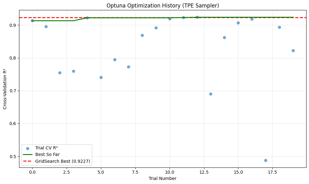
Trials needed to match GridSearch: 12/20

Understanding the Hyperparameter Landscape

Optuna provides built-in visualizations to understand which parameters matter most.

from optuna.visualization import plot_param_importances, plot_contour

# Parameter importance (based on functional ANOVA)
fig = plot_param_importances(study)
fig.update_layout(title='Which Hyperparameter Matters More?')
fig.show()

print("\nInterpretation:")
print("- Higher importance = larger impact on CV score")
print("- In this sparse regression problem, both alpha and l1_ratio matter")
print("- Alpha controls overall regularization strength")
print("- L1_ratio controls feature selection (higher = more Lasso-like)")

# Contour plot: alpha vs l1_ratio landscape
fig = plot_contour(study, params=['alpha', 'l1_ratio'])
fig.update_layout(title='Hyperparameter Landscape: Alpha vs L1 Ratio')
fig.show()

print("\nCompare to GridSearchCV heatmap (Cell 25):")
print("- GridSearch samples uniformly (20 fixed grid points)")
print("- Optuna samples densely in promising regions (adaptive)")
print("- Both identify similar optimal region (low-to-medium alpha, high l1_ratio)")

Interpretation:
- Higher importance = larger impact on CV score
- In this sparse regression problem, both alpha and l1_ratio matter
- Alpha controls overall regularization strength
- L1_ratio controls feature selection (higher = more Lasso-like)

Compare to GridSearchCV heatmap (Cell 25):
- GridSearch samples uniformly (20 fixed grid points)
- Optuna samples densely in promising regions (adaptive)
- Both identify similar optimal region (low-to-medium alpha, high l1_ratio)

Advanced: Automatic Model Selection

GridSearchCV can’t easily compare different model types. Optuna can suggest categorical choices, enabling model architecture search.

def multi_model_objective(trial):
    """
    Objective that selects model type AND tunes its hyperparameters.
    
    Demonstrates categorical parameters and conditional logic.
    """
    # Suggest model type
    model_type = trial.suggest_categorical('model', ['Ridge', 'Lasso', 'ElasticNet'])
    
    # Shared hyperparameter
    alpha = trial.suggest_float('alpha', 0.001, 10.0, log=True)
    
    # Model-specific hyperparameters
    if model_type == 'Ridge':
        from sklearn.linear_model import Ridge
        model = Ridge(alpha=alpha)
    elif model_type == 'Lasso':
        from sklearn.linear_model import Lasso
        model = Lasso(alpha=alpha, max_iter=10000)
    else:  # ElasticNet
        l1_ratio = trial.suggest_float('l1_ratio', 0.1, 0.9)
        model = ElasticNet(alpha=alpha, l1_ratio=l1_ratio, max_iter=10000)
    
    # Evaluate
    scores = cross_val_score(model, X_train, y_train, cv=5, scoring='r2')
    return scores.mean()

# Optimize with larger budget (3 models to explore)
multi_study = optuna.create_study(direction='maximize', sampler=optuna.samplers.TPESampler(seed=42))
multi_study.optimize(multi_model_objective, n_trials=30)

print("Best Configuration:")
print(f"  Model: {multi_study.best_params['model']}")
print(f"  Alpha: {multi_study.best_params['alpha']:.4f}")
if 'l1_ratio' in multi_study.best_params:
    print(f"  L1 Ratio: {multi_study.best_params['l1_ratio']:.4f}")
print(f"  CV R²: {multi_study.best_value:.4f}")

# Count model selections
model_counts = {}
for trial in multi_study.trials:
    model = trial.params['model']
    model_counts[model] = model_counts.get(model, 0) + 1

print(f"\nModel Selection Frequency:")
for model, count in sorted(model_counts.items(), key=lambda x: x[1], reverse=True):
    print(f"  {model}: {count}/{len(multi_study.trials)} trials ({100*count/len(multi_study.trials):.1f}%)")

print("\nNote: This is difficult/impossible with GridSearchCV!")
print("You'd need separate grid searches for each model type.")

Best Configuration:
  Model: Lasso
  Alpha: 0.0349
  CV R²: 0.9317

Model Selection Frequency:
  Lasso: 20/30 trials (66.7%)
  Ridge: 5/30 trials (16.7%)
  ElasticNet: 5/30 trials (16.7%)

Note: This is difficult/impossible with GridSearchCV!
You'd need separate grid searches for each model type.

Optuna + Pipelines: Production Pattern

Combine Optuna with scikit-learn pipelines for a complete, leak-free workflow.

from sklearn.pipeline import Pipeline
from sklearn.preprocessing import StandardScaler

def pipeline_objective(trial):
    """
    Tune preprocessing AND model hyperparameters together.
    
    Demonstrates that Optuna works seamlessly with Pipeline objects.
    """
    # Preprocessing choices
    use_scaling = trial.suggest_categorical('use_scaling', [True, False])
    
    # Model hyperparameters
    alpha = trial.suggest_float('alpha', 0.001, 1.0, log=True)
    l1_ratio = trial.suggest_float('l1_ratio', 0.1, 0.9)
    
    # Build pipeline
    steps = []
    if use_scaling:
        steps.append(('scaler', StandardScaler()))
    steps.append(('model', ElasticNet(alpha=alpha, l1_ratio=l1_ratio, max_iter=10000)))
    
    pipeline = Pipeline(steps)
    
    # Evaluate (cross_val_score handles train/val splits correctly, no leakage)
    scores = cross_val_score(pipeline, X_train, y_train, cv=5, scoring='r2')
    return scores.mean()

# Optimize
pipeline_study = optuna.create_study(direction='maximize', sampler=optuna.samplers.TPESampler(seed=42))
pipeline_study.optimize(pipeline_objective, n_trials=20)

print("Best Pipeline Configuration:")
print(f"  Use Scaling: {pipeline_study.best_params['use_scaling']}")
print(f"  Alpha: {pipeline_study.best_params['alpha']:.4f}")
print(f"  L1 Ratio: {pipeline_study.best_params['l1_ratio']:.4f}")
print(f"  CV R²: {pipeline_study.best_value:.4f}")

print("\nNote: Regularization typically requires scaling (penalizes by magnitude).")
print("Optuna should discover use_scaling=True is better.")
print("This demonstrates automatic discovery of preprocessing choices!")

Best Pipeline Configuration:
  Use Scaling: True
  Alpha: 0.0512
  L1 Ratio: 0.7884
  CV R²: 0.9294

Note: Regularization typically requires scaling (penalizes by magnitude).
Optuna should discover use_scaling=True is better.
This demonstrates automatic discovery of preprocessing choices!

Summary: When to Use Optuna

Advantages:

• Smarter sampling: TPE learns from past trials, focuses on promising regions

• Continuous spaces: No need to discretize (alpha can be any value in [0.001, 1.0])

• Scalability: Efficient with many hyperparameters (>3 dimensions)

• Flexibility: Categorical choices, conditional parameters, multi-model selection

• Transparency: Built-in visualizations and importance analysis

Limitations:

• External dependency: Not in scikit-learn, requires installation

• Complexity: More code than GridSearchCV for simple cases

• Randomness: Non-deterministic (even with seed, results may vary slightly)

• Overhead: For tiny search spaces (<20 trials), GridSearch is simpler

Best Practices:

1. Start with GridSearch for initial exploration (discrete, interpretable)

2. Switch to Optuna when:

   • Search space is large (>50 combinations)

   • Hyperparameters are continuous

   • You need to compare different model architectures

3. Use the same CV strategy for fair comparison (same folds, same metric)

4. Set a seed for reproducibility (sampler=TPESampler(seed=42))

5. Visualize the optimization to ensure convergence

6. Combine with Pipelines to prevent data leakage

Alternative Tools:

• scikit-learn’s RandomizedSearchCV: Middle ground (random sampling, no Bayesian optimization)

• Hyperopt: Similar to Optuna, TPE-based (Optuna has cleaner API)

• Ray Tune: For distributed hyperparameter search at scale

• Weights & Biases Sweeps: For deep learning experiment tracking

Key Takeaway

GridSearchCV is exhaustive and interpretable. Optuna is intelligent and efficient. For most problems, start with GridSearchCV. Upgrade to Optuna when you need more power, flexibility, or efficiency.

---

Pipelines for Reproducible Workflows

Combine preprocessing and modeling into a single pipeline.

# Pipeline example
pipeline = Pipeline([
    ('scaler', StandardScaler()),
    ('poly', PolynomialFeatures(degree=2, include_bias=False)),
    ('lasso', Lasso(alpha=0.1, max_iter=10000))
])

# Cross-validate the entire pipeline
scores = cross_val_score(pipeline, X, y, cv=5, scoring='r2')
print(f"Pipeline CV R²: {scores.mean():.4f} (+/- {scores.std()*2:.4f})")

Pipeline CV R²: 0.9226 (+/- 0.0631)

# Grid search with pipeline
pipeline = Pipeline([
    ('scaler', StandardScaler()),
    ('model', Ridge())
])

param_grid = {
    'model__alpha': np.logspace(-2, 4, 20)
}

grid = GridSearchCV(pipeline, param_grid, cv=5, scoring='r2')
grid.fit(X_train, y_train)

print(f"Best alpha: {grid.best_params_['model__alpha']:.4f}")
print(f"Test R²: {grid.score(X_test, y_test):.4f}")

Best alpha: 1.6238
Test R²: 0.8655

Model Comparison Summary

# Compare all methods
models = {
    'OLS': LinearRegression(),
    'Ridge (CV)': RidgeCV(alphas=np.logspace(-4, 4, 50), cv=5),
    'Lasso (CV)': LassoCV(alphas=np.logspace(-4, 1, 50), cv=5, max_iter=10000),
    'ElasticNet (CV)': ElasticNetCV(l1_ratio=[0.1, 0.5, 0.9], cv=5, max_iter=10000)
}

results = []
for name, model in models.items():
    model.fit(X_train, y_train)
    train_score = model.score(X_train, y_train)
    test_score = model.score(X_test, y_test)
    
    # Count non-zero coefficients
    n_nonzero = np.sum(model.coef_ != 0)
    
    results.append({
        'Model': name,
        'Train R²': train_score,
        'Test R²': test_score,
        'Overfit Gap': train_score - test_score,
        'Non-zero Coefs': n_nonzero
    })

results_df = pd.DataFrame(results)
print(results_df.to_string(index=False))

          Model  Train R²  Test R²  Overfit Gap  Non-zero Coefs
            OLS  0.992675 0.888357     0.104318              50
     Ridge (CV)  0.991720 0.876808     0.114912              50
     Lasso (CV)  0.984205 0.966050     0.018155              31
ElasticNet (CV)  0.985114 0.964101     0.021013              31

Test Your Knowledge

%pip install -q jupyterquiz
from jupyterquiz import display_quiz

display_quiz("https://raw.githubusercontent.com/jkitchin/s26-06642/main/dsmles/08-regularization-model-selection/quizzes/regularization-quiz.json")

Note: you may need to restart the kernel to use updated packages.

Recommended Reading

These resources cover regularization theory and model selection best practices:

1. An Introduction to Statistical Learning, Chapter 6 - Comprehensive coverage of Ridge, Lasso, and model selection. Includes the geometric intuition for why L1 produces sparsity.

2. Scikit-learn Model Selection - Official documentation on cross-validation, grid search, and hyperparameter tuning. Essential reference for practical implementation.

3. Regularization for Machine Learning (Ng, Stanford CS229) - Course notes explaining the bias-variance tradeoff and how regularization addresses overfitting. Clear mathematical treatment.

4. The Elements of Statistical Learning, Chapter 3 - Advanced treatment of shrinkage methods including the relationship between Ridge, Lasso, and subset selection. Free PDF available.

5. Cross-Validation Pitfalls (Hastie & Efron) - Discusses common mistakes in cross-validation, including data leakage and proper nested CV. Important for avoiding subtle errors.

Summary: Regularization and Model Selection

The Regularization Toolkit

Method	Penalty	Effect	Use When
Ridge	L2 (squared)	Shrinks all coefficients	Multicollinearity, stability
Lasso	L1 (absolute)	Some coefficients = 0	Feature selection, sparsity
ElasticNet	L1 + L2	Combines both	Correlated features + selection

Key Decisions

Decision	Guidance
Ridge vs Lasso?	Lasso if you want feature selection; Ridge if all features might matter
How to choose α?	Cross-validation (RidgeCV, LassoCV)
How many folds?	5-10 is typical
Grid search exhaustive?	Use RandomizedSearchCV for many hyperparameters

The Model Selection Workflow

1. Start with cross-validation for reliable estimates

2. *Use CV variants (RidgeCV, LassoCV) for automatic hyperparameter tuning

3. Use GridSearchCV when you have multiple hyperparameters

4. Use Pipelines to combine preprocessing + modeling + tuning

Common Pitfalls

• Tuning on test data: Never! Use cross-validation for tuning, keep test set for final evaluation

• Forgetting to scale: Regularization penalizes magnitude—scale features first!

• Ignoring ElasticNet: It’s often better than pure Lasso with correlated features

• Not using pipelines: Risk of data leakage when scaling/transforming

Next Steps

In the next module, we’ll explore nonlinear methods (polynomial features, SVR) for when linear models aren’t enough.

---

The Catalyst Crisis: Chapter 8 - “The Danger of Being Too Clever”

A story about overfitting, regularization, and learning from struggle

---

Jordan was still in the lab at 11 PM when Alex arrived.

He startled at the door. “I didn’t hear you come in.”

“Couldn’t sleep. Thought I’d review some results.” Alex noticed the dark circles under Jordan’s eyes, the forest of crumpled sticky notes around his laptop. “How long have you been here?”

“I don’t know. A while.” He gestured at his screen. “I built this model—polynomial features, degree four, all the interactions. R-squared of 0.97 on training data.”

Alex sat down beside him. “What about test data?”

Jordan was silent for a moment. “0.41.”

“Ah.”

“I don’t understand. It fits the training data almost perfectly. But when I give it new data…” He trailed off.

Alex had made this exact mistake, three weeks ago. It was strangely comforting to see someone else struggling with it too.

“You’re overfitting,” she said gently. “The model memorized the training data instead of learning the underlying pattern. It’s like studying for a test by memorizing the answers to last year’s questions. Works great until the questions change.”

“So what do I do?”

“Regularization.” Alex pulled up her own work. “Ridge and Lasso. They add a penalty for model complexity. The model has to earn each feature—if a variable isn’t pulling its weight, it gets shrunk toward zero.”

They worked together through the night, rebuilding Jordan’s model with L1 regularization. The training R-squared dropped to 0.82—less impressive on paper. But the test R-squared climbed to 0.79. The gap nearly closed.

“It’s… less good on training data,” Jordan said uncertainly.

“But more honest. More generalizable.” Alex pointed at the coefficient plot. “Look—Lasso zeroed out twenty features. They weren’t helping; they were fitting noise.”

“How do you know which features to trust?”

“The ones that survive regularization. The ones that show up consistently across cross-validation folds. The ones that make physical sense.” She highlighted the non-zero coefficients. “Catalyst age. Temperature. Pressure. The basics. Everything else was distraction.”

Jordan leaned back, exhaustion and relief mingling on his face. “You too? The struggling, I mean?”

“Everyone. Maya’s been up late debugging. Sam nearly quit after their PCA mistake. We’re all figuring it out.”

“Nobody talks about it.”

“I know. We should.” Alex stood to leave, then paused. “Same time tomorrow? I’m working on the classification threshold problem—could use a second set of eyes.”

Jordan nodded. “Thanks, Alex.”

She added to the mystery board: Simpler models generalize better. Regularization keeps only what matters: catalyst, temperature, pressure.

---

Continue to the next lecture to explore nonlinear methods…