Module 02: Pandas Introduction

Module 02: Pandas Introduction#

Pandas provides high-level data structures for working with tabular (spreadsheet-like) data.

Learning Objectives#

Create and manipulate DataFrames and Series
Load data from CSV, Excel, and other formats
Select and filter data
Handle missing values
Create basic visualizations

import pandas as pd
import numpy as np
import matplotlib.pyplot as plt

Why Pandas? From Arrays to Labeled Data#

NumPy is powerful, but it has limitations for real-world data:

No column names: You have to remember that column 0 is temperature, column 1 is pressure…
No mixed types: Can’t have strings and numbers in the same array
No built-in missing data: NaN handling is awkward
No metadata: Dates, categories, and units need manual tracking

Enter Pandas#

Pandas provides two main data structures:

Series: A labeled 1D array (like a column in a spreadsheet)
DataFrame: A labeled 2D table (like an entire spreadsheet)

The key innovation is labels. Instead of accessing data by position (data[0, 2]), you access it by name (data['temperature']). This makes code more readable and less error-prone.

When to Use Pandas vs NumPy#

Use Pandas when…	Use NumPy when…
You have tabular data with column names	You need raw numerical performance
You need to join/merge datasets	You’re doing linear algebra
You have mixed types (strings + numbers)	You’re implementing algorithms
You need to handle missing data	You’re building ML model internals
You’re exploring and cleaning data	You’re doing image processing

In practice, you’ll often use both: Pandas for data wrangling, then extract NumPy arrays for modeling.

# Create a Series
temperatures = pd.Series([300, 350, 400, 450, 500], name='temperature')
print(temperatures)
print("\nType:", type(temperatures))

  300
  350
  400
  450
  500
Name: temperature, dtype: int64

Type: <class 'pandas.Series'>

# Create a DataFrame from a dictionary
data = {
    'temperature': [300, 350, 400, 450, 500],
    'pressure': [1.0, 1.5, 2.0, 2.5, 3.0],
    'catalyst': ['Pt', 'Pt', 'Pd', 'Pd', 'Pt'],
    'yield': [45.2, 52.8, 68.1, 75.4, 82.0]
}

df = pd.DataFrame(data)
df

	temperature	pressure	catalyst	yield
0	300	1.0	Pt	45.2
1	350	1.5	Pt	52.8
2	400	2.0	Pd	68.1
3	450	2.5	Pd	75.4
4	500	3.0	Pt	82.0

# Basic DataFrame info
print("Shape:", df.shape)
print("\nColumns:", df.columns.tolist())
print("\nData types:")
print(df.dtypes)

Shape: (5, 4)

Columns: ['temperature', 'pressure', 'catalyst', 'yield']

Data types:
temperature      int64
pressure       float64
catalyst           str
yield          float64
dtype: object

# Quick summary statistics
df.describe()

	temperature	pressure	yield
count	5.000000	5.000000	5.000000
mean	400.000000	2.000000	64.700000
std	79.056942	0.790569	15.388307
min	300.000000	1.000000	45.200000
25%	350.000000	1.500000	52.800000
50%	400.000000	2.000000	68.100000
75%	450.000000	2.500000	75.400000
max	500.000000	3.000000	82.000000

Loading Data: Your Gateway to Real Datasets#

In real work, you rarely create DataFrames from scratch. Instead, you load data from files, databases, or web APIs. Pandas makes this remarkably easy.

The Most Common Scenario: CSV Files#

CSV (Comma-Separated Values) is the universal exchange format for tabular data. Every instrument, database, and software can export CSV. This is often your first step:

df = pd.read_csv('my_data.csv')

What Can Go Wrong?#

Real data is messy. Here are common issues and how Pandas handles them:

Problem	Solution
Wrong delimiter (tabs, semicolons)	`sep='\t'` or `sep=';'`
Header on wrong row	`header=2` (0-indexed)
Missing values coded as text	`na_values=['NA', 'missing', '-']`
Too large to fit in memory	`usecols=['temp', 'yield']` or `nrows=1000`
Encoding issues (accented characters)	`encoding='utf-8'` or `'latin-1'`

Pro tip: Always inspect your data immediately after loading with df.head(), df.info(), and df.describe(). Catch problems early!

# Create sample data file
sample_data = """experiment_id,temperature,pressure,catalyst,conversion,selectivity,notes
EXP001,300,1.0,Pt/Al2O3,0.45,0.92,baseline
EXP002,350,1.0,Pt/Al2O3,0.58,0.89,
EXP003,400,1.0,Pt/Al2O3,0.72,0.85,
EXP004,400,2.0,Pt/Al2O3,0.78,0.83,high pressure
EXP005,400,1.0,Pd/Al2O3,0.65,0.91,different catalyst
EXP006,450,1.0,Pt/Al2O3,0.81,0.79,
EXP007,450,1.5,Pt/Al2O3,0.85,0.77,
EXP008,500,1.0,Pt/Al2O3,0.89,0.71,high temp
EXP009,500,1.0,Pd/Al2O3,,0.82,catalyst test - no conversion data
EXP010,350,1.0,Pt/Al2O3,0.57,0.90,replicate of EXP002
"""

with open('experiments.csv', 'w') as f:
    f.write(sample_data)

# Load CSV
df = pd.read_csv('experiments.csv')
df

	experiment_id	temperature	pressure	catalyst	conversion	selectivity	notes
0	EXP001	300	1.0	Pt/Al2O3	0.45	0.92	baseline
1	EXP002	350	1.0	Pt/Al2O3	0.58	0.89	NaN
2	EXP003	400	1.0	Pt/Al2O3	0.72	0.85	NaN
3	EXP004	400	2.0	Pt/Al2O3	0.78	0.83	high pressure
4	EXP005	400	1.0	Pd/Al2O3	0.65	0.91	different catalyst
5	EXP006	450	1.0	Pt/Al2O3	0.81	0.79	NaN
6	EXP007	450	1.5	Pt/Al2O3	0.85	0.77	NaN
7	EXP008	500	1.0	Pt/Al2O3	0.89	0.71	high temp
8	EXP009	500	1.0	Pd/Al2O3	NaN	0.82	catalyst test - no conversion data
9	EXP010	350	1.0	Pt/Al2O3	0.57	0.90	replicate of EXP002

# Useful read_csv options:
# pd.read_csv('file.csv', 
#     sep=',',           # Delimiter
#     header=0,          # Row number for column names
#     index_col=0,       # Column to use as index
#     usecols=[0,1,2],   # Only load specific columns
#     nrows=100,         # Only load first N rows
#     skiprows=5,        # Skip first N rows
#     na_values=['NA', 'missing']  # Values to treat as NaN
# )

# Other formats:
# pd.read_excel('file.xlsx')
# pd.read_json('file.json')
# pd.read_sql('SELECT * FROM table', connection)

Selecting Data: The Core Skill#

Data selection is what you’ll do most often in Pandas. There are multiple ways to select data, and choosing the right one matters:

The Selection Zoo#

Syntax	What it does	Returns
`df['col']`	Select one column	Series
`df[['col1', 'col2']]`	Select multiple columns	DataFrame
`df.iloc[0]`	Select row by position	Series
`df.iloc[0:5]`	Select rows by position range	DataFrame
`df.loc['label']`	Select row by index label	Series
`df[df['col'] > 5]`	Filter rows by condition	DataFrame

The Most Powerful Pattern: Boolean Filtering#

This is the pattern you’ll use most often:

df[condition]  # Returns rows where condition is True

Conditions can be combined with & (and), | (or), and ~ (not). Always wrap each condition in parentheses:

df[(df['temp'] > 400) & (df['pressure'] < 5)]

Common Mistake: `and` vs `&`#

Python’s and doesn’t work with Pandas! Use & instead. This is because Pandas needs to apply the operation element-wise.

# Select a column (returns Series)
df['temperature']

  300
  350
  400
  400
  400
  450
  450
  500
  500
  350
Name: temperature, dtype: int64

# Select multiple columns (returns DataFrame)
df[['temperature', 'conversion', 'selectivity']]

	temperature	conversion	selectivity
0	300	0.45	0.92
1	350	0.58	0.89
2	400	0.72	0.85
3	400	0.78	0.83
4	400	0.65	0.91
5	450	0.81	0.79
6	450	0.85	0.77
7	500	0.89	0.71
8	500	NaN	0.82
9	350	0.57	0.90

# Select rows by position with .iloc
print("First row:")
print(df.iloc[0])

print("\nFirst 3 rows:")
print(df.iloc[:3])

First row:
experiment_id      EXP001
temperature           300
pressure              1.0
catalyst         Pt/Al2O3
conversion           0.45
selectivity          0.92
notes            baseline
Name: 0, dtype: object

First 3 rows:
  experiment_id  temperature  pressure  catalyst  conversion  selectivity  \
0        EXP001          300       1.0  Pt/Al2O3        0.45         0.92   
1        EXP002          350       1.0  Pt/Al2O3        0.58         0.89   
2        EXP003          400       1.0  Pt/Al2O3        0.72         0.85   

      notes  
0  baseline  
1       NaN  
2       NaN  

# Select rows by label with .loc
df_indexed = df.set_index('experiment_id')
print(df_indexed.loc['EXP003'])

temperature         400
pressure            1.0
catalyst       Pt/Al2O3
conversion         0.72
selectivity        0.85
notes               NaN
Name: EXP003, dtype: object

# Boolean filtering - most common in practice!
# Find high-temperature experiments
high_temp = df[df['temperature'] >= 400]
high_temp

	experiment_id	temperature	pressure	catalyst	conversion	selectivity	notes
2	EXP003	400	1.0	Pt/Al2O3	0.72	0.85	NaN
3	EXP004	400	2.0	Pt/Al2O3	0.78	0.83	high pressure
4	EXP005	400	1.0	Pd/Al2O3	0.65	0.91	different catalyst
5	EXP006	450	1.0	Pt/Al2O3	0.81	0.79	NaN
6	EXP007	450	1.5	Pt/Al2O3	0.85	0.77	NaN
7	EXP008	500	1.0	Pt/Al2O3	0.89	0.71	high temp
8	EXP009	500	1.0	Pd/Al2O3	NaN	0.82	catalyst test - no conversion data

# Multiple conditions (use & for AND, | for OR)
# High temp AND high conversion
subset = df[(df['temperature'] >= 400) & (df['conversion'] > 0.7)]
subset

	experiment_id	temperature	pressure	catalyst	conversion	selectivity	notes
2	EXP003	400	1.0	Pt/Al2O3	0.72	0.85	NaN
3	EXP004	400	2.0	Pt/Al2O3	0.78	0.83	high pressure
5	EXP006	450	1.0	Pt/Al2O3	0.81	0.79	NaN
6	EXP007	450	1.5	Pt/Al2O3	0.85	0.77	NaN
7	EXP008	500	1.0	Pt/Al2O3	0.89	0.71	high temp

# Filter by categorical values
pt_experiments = df[df['catalyst'] == 'Pt/Al2O3']
print(f"Pt experiments: {len(pt_experiments)}")

# Filter by multiple values
selected_temps = df[df['temperature'].isin([300, 400, 500])]
selected_temps

Pt experiments: 8

	experiment_id	temperature	pressure	catalyst	conversion	selectivity	notes
0	EXP001	300	1.0	Pt/Al2O3	0.45	0.92	baseline
2	EXP003	400	1.0	Pt/Al2O3	0.72	0.85	NaN
3	EXP004	400	2.0	Pt/Al2O3	0.78	0.83	high pressure
4	EXP005	400	1.0	Pd/Al2O3	0.65	0.91	different catalyst
7	EXP008	500	1.0	Pt/Al2O3	0.89	0.71	high temp
8	EXP009	500	1.0	Pd/Al2O3	NaN	0.82	catalyst test - no conversion data

Handling Missing Data: The Unavoidable Reality#

Real experimental data almost always has missing values. Sensors fail, experiments are interrupted, data entry has errors. Pandas uses NaN (Not a Number) to represent missing data.

Why Missing Data Matters#

Many operations fail or give wrong results with missing data:

Mean of [1, 2, NaN] could be 1.5 or undefined
ML models often can’t handle NaN
Joins may drop rows unexpectedly

Strategies for Missing Data#

There’s no universal solution—the right choice depends on why the data is missing:

Strategy	When to Use	Pandas Method
Drop rows	Data is missing randomly, you have plenty of data	`df.dropna()`
Drop columns	A column has too many missing values to be useful	`df.drop(columns=['col'])`
Fill with constant	You have a meaningful default value	`df.fillna(0)`
Fill with mean/median	Missing at random, want to preserve distribution	`df.fillna(df.mean())`
Forward fill	Time series where last value carries forward	`df.ffill()`
Interpolate	Time series with gradual changes	`df.interpolate()`

The Key Question#

Before choosing a strategy, ask: Why is this data missing?

Missing Completely at Random (MCAR): Sensor battery died → safe to drop or impute
Missing at Random (MAR): High-temp experiments failed more often → imputation may bias results
Missing Not at Random (MNAR): Conversion too low to measure → dropping creates selection bias

For MNAR data, no simple fix works. You may need domain expertise or more sophisticated methods.

# Check for missing values
print("Missing values per column:")
print(df.isna().sum())

print("\nRows with any missing values:")
print(df[df.isna().any(axis=1)])

Missing values per column:
experiment_id    0
temperature      0
pressure         0
catalyst         0
conversion       1
selectivity      0
notes            4
dtype: int64

Rows with any missing values:
  experiment_id  temperature  pressure  catalyst  conversion  selectivity  \
1        EXP002          350       1.0  Pt/Al2O3        0.58         0.89   
2        EXP003          400       1.0  Pt/Al2O3        0.72         0.85   
5        EXP006          450       1.0  Pt/Al2O3        0.81         0.79   
6        EXP007          450       1.5  Pt/Al2O3        0.85         0.77   
8        EXP009          500       1.0  Pd/Al2O3         NaN         0.82   

                                notes  
1                                 NaN  
2                                 NaN  
5                                 NaN  
6                                 NaN  
8  catalyst test - no conversion data  

# Options for handling missing data

# 1. Drop rows with missing values
df_dropped = df.dropna()
print(f"Original: {len(df)} rows, After dropna: {len(df_dropped)} rows")

# 2. Drop only if specific columns are missing
df_dropped2 = df.dropna(subset=['conversion'])

# 3. Fill with a value
df_filled = df.fillna({'conversion': df['conversion'].mean()})

# 4. Forward fill (useful for time series)
# df_ffill = df.fillna(method='ffill')

Original: 10 rows, After dropna: 5 rows

Adding and Modifying Columns#

# Create a working copy
df_work = df.copy()

# Add a calculated column
df_work['yield'] = df_work['conversion'] * df_work['selectivity'] * 100

# Add temperature in Celsius
df_work['temp_C'] = df_work['temperature'] - 273.15

df_work[['experiment_id', 'temperature', 'temp_C', 'conversion', 'selectivity', 'yield']]

	experiment_id	temperature	temp_C	conversion	selectivity	yield
0	EXP001	300	26.85	0.45	0.92	41.40
1	EXP002	350	76.85	0.58	0.89	51.62
2	EXP003	400	126.85	0.72	0.85	61.20
3	EXP004	400	126.85	0.78	0.83	64.74
4	EXP005	400	126.85	0.65	0.91	59.15
5	EXP006	450	176.85	0.81	0.79	63.99
6	EXP007	450	176.85	0.85	0.77	65.45
7	EXP008	500	226.85	0.89	0.71	63.19
8	EXP009	500	226.85	NaN	0.82	NaN
9	EXP010	350	76.85	0.57	0.90	51.30

# Categorize based on conditions
def classify_temp(temp):
    if temp < 350:
        return 'low'
    elif temp < 450:
        return 'medium'
    else:
        return 'high'

df_work['temp_category'] = df_work['temperature'].apply(classify_temp)
df_work[['experiment_id', 'temperature', 'temp_category']]

	experiment_id	temperature	temp_category
0	EXP001	300	low
1	EXP002	350	medium
2	EXP003	400	medium
3	EXP004	400	medium
4	EXP005	400	medium
5	EXP006	450	high
6	EXP007	450	high
7	EXP008	500	high
8	EXP009	500	high
9	EXP010	350	medium

Basic Visualization with Pandas#

# Scatter plot
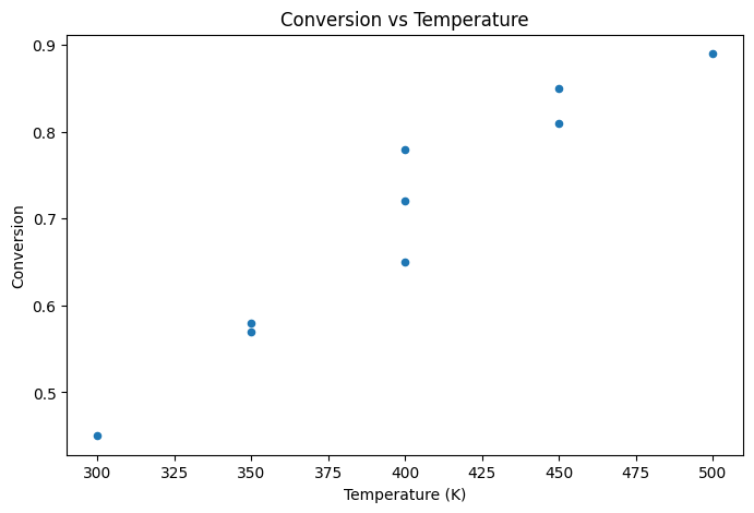
df.plot.scatter(x='temperature', y='conversion', figsize=(8, 5))
plt.xlabel('Temperature (K)')
plt.ylabel('Conversion')
plt.title('Conversion vs Temperature')
plt.show()

../_images/774a543d26cd6b5f0cc1765dcb9c87f9d11199fffd476b41377a82be544aeb89.png

# Histogram
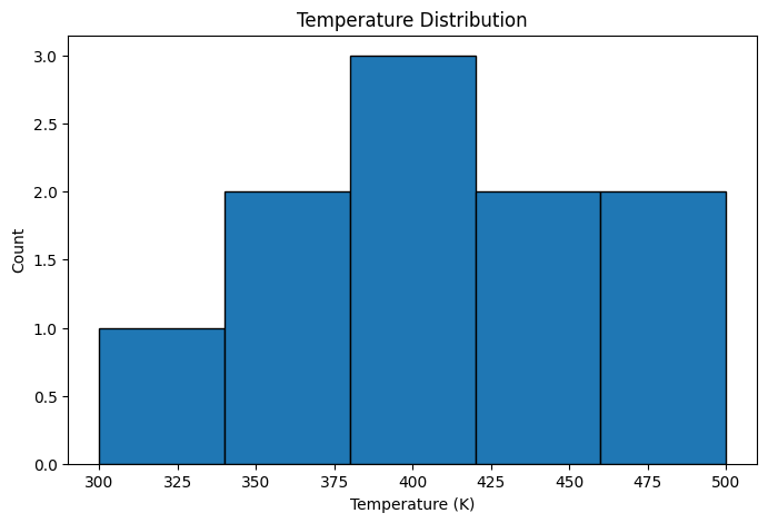
df['temperature'].plot.hist(bins=5, edgecolor='black', figsize=(8, 5))
plt.xlabel('Temperature (K)')
plt.ylabel('Count')
plt.title('Temperature Distribution')
plt.show()

../_images/94bcbd1a4833fec50c7d6367ac5bde4e6b93bcd2fdf44c2327ae76cb47bb9dc1.png

# Box plot by category
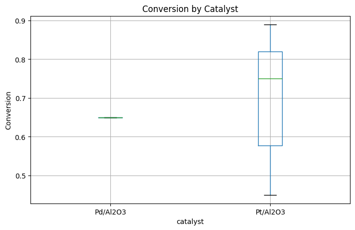
df.boxplot(column='conversion', by='catalyst', figsize=(8, 5))
plt.ylabel('Conversion')
plt.title('Conversion by Catalyst')
plt.suptitle('')  # Remove automatic title
plt.show()

../_images/186fd24e2ff49afe14574dd92f5ce0a7078b2423f9724b627bad80d2a001ac51.png

Sorting and Ranking#

# Sort by one column
df.sort_values('conversion', ascending=False)

	experiment_id	temperature	pressure	catalyst	conversion	selectivity	notes
7	EXP008	500	1.0	Pt/Al2O3	0.89	0.71	high temp
6	EXP007	450	1.5	Pt/Al2O3	0.85	0.77	NaN
5	EXP006	450	1.0	Pt/Al2O3	0.81	0.79	NaN
3	EXP004	400	2.0	Pt/Al2O3	0.78	0.83	high pressure
2	EXP003	400	1.0	Pt/Al2O3	0.72	0.85	NaN
4	EXP005	400	1.0	Pd/Al2O3	0.65	0.91	different catalyst
1	EXP002	350	1.0	Pt/Al2O3	0.58	0.89	NaN
9	EXP010	350	1.0	Pt/Al2O3	0.57	0.90	replicate of EXP002
0	EXP001	300	1.0	Pt/Al2O3	0.45	0.92	baseline
8	EXP009	500	1.0	Pd/Al2O3	NaN	0.82	catalyst test - no conversion data

# Sort by multiple columns
df.sort_values(['catalyst', 'temperature'])

	experiment_id	temperature	pressure	catalyst	conversion	selectivity	notes
4	EXP005	400	1.0	Pd/Al2O3	0.65	0.91	different catalyst
8	EXP009	500	1.0	Pd/Al2O3	NaN	0.82	catalyst test - no conversion data
0	EXP001	300	1.0	Pt/Al2O3	0.45	0.92	baseline
1	EXP002	350	1.0	Pt/Al2O3	0.58	0.89	NaN
9	EXP010	350	1.0	Pt/Al2O3	0.57	0.90	replicate of EXP002
2	EXP003	400	1.0	Pt/Al2O3	0.72	0.85	NaN
3	EXP004	400	2.0	Pt/Al2O3	0.78	0.83	high pressure
5	EXP006	450	1.0	Pt/Al2O3	0.81	0.79	NaN
6	EXP007	450	1.5	Pt/Al2O3	0.85	0.77	NaN
7	EXP008	500	1.0	Pt/Al2O3	0.89	0.71	high temp

# Get top/bottom N
print("Top 3 by conversion:")
df.nlargest(3, 'conversion')

Top 3 by conversion:

	experiment_id	temperature	pressure	catalyst	conversion	selectivity	notes
7	EXP008	500	1.0	Pt/Al2O3	0.89	0.71	high temp
6	EXP007	450	1.5	Pt/Al2O3	0.85	0.77	NaN
5	EXP006	450	1.0	Pt/Al2O3	0.81	0.79	NaN

Saving Data#

# Save to CSV
df_work.to_csv('experiments_processed.csv', index=False)

# Other formats:
# df_work.to_excel('experiments.xlsx', index=False)
# df_work.to_json('experiments.json')

print("Data saved!")

Data saved!

The Catalyst Crisis: “The Ghost in the Data”#

Continued from NumPy…

“Fifteen percent of the temperature readings are missing,” Alex announced to her study group. “And I know why.”

Jordan looked up from his laptop, interested for the first time all week. Sam didn’t look up at all, fingers flying across their keyboard.

“Shift changes,” Alex continued. “The gaps cluster at 11 PM, 3 AM, and 7 AM. Operators are supposed to log backup readings when sensors drop out, but during handoffs, it’s getting missed.”

Maya frowned. “So we just… fill them in? Take the average?”

“That’s what I thought initially.” Alex pulled up a visualization she’d built—a heatmap showing missing values by time and reactor conditions. “But look at this. The missingness isn’t random. It correlates with high-temperature excursions.”

Jordan leaned in. “The sensors are dropping out precisely when things get interesting.”

“Exactly. If we just fill in the mean, we’re erasing exactly the moments that might matter most.”

Sam finally looked up. “So what do you do?”

Alex hesitated. This was the part she wasn’t sure about. “I think… the missing data itself is information. We shouldn’t just fill it in. We should flag it. Track which batches have missing readings during high-temperature events.”

“That’s a lot of extra work,” Sam said.

“It’s the right extra work.”

That afternoon, Frank Morrison—ChemCorp’s process engineer and the Academy’s industrial liaison—joined their virtual meeting. He had the skeptical look of someone who’d seen too many consultants come and go.

“So you’ve spent a week looking at missing data,” he said. “We knew the sensors were unreliable. What’s new?”

Alex took a breath. “The sensors fail during temperature excursions. Which means your worst batches—the ones you most need to understand—are the ones with the least data.”

Frank was quiet for a moment. “Huh. We always assumed the sensor failures were random.”

“They’re not. And I think that’s a clue.”

After the call, Jordan caught Alex in the hallway. “That was good. The way you pushed back.”

“I wasn’t sure I should.”

“You had evidence. That’s all the permission you need.”

Alex added to the mystery board: Missing data correlates with temperature excursions. Sensor failures aren’t random—they’re symptoms.

To be continued…

Quiz: Test Your Understanding#

Test your knowledge of the Pandas concepts covered in this module.

%pip install -q jupyterquiz
from jupyterquiz import display_quiz

display_quiz("https://raw.githubusercontent.com/jkitchin/s26-06642/main/dsmles/02-pandas-intro/quizzes/pandas-intro-quiz.json")

Note: you may need to restart the kernel to use updated packages.

Summary: The Pandas Mental Model#

Pandas is your data wrangling workbench. Here’s how to think about it:

Core Concepts#

Concept	Key Idea	Chemical Engineering Example
DataFrame	Labeled 2D table	Experiment log with conditions and results
Series	Labeled 1D array	A column of temperature measurements
Index	Row labels	Experiment IDs or timestamps
Selection	Filter by condition	Find high-conversion experiments

The Typical Workflow#

Load: pd.read_csv('data.csv')
Inspect: df.head(), df.info(), df.describe()
Clean: Handle missing values, fix data types
Transform: Add columns, filter rows
Analyze: Compute statistics, visualize
Export: df.to_csv('cleaned_data.csv')

Key Takeaways#

Labels > positions: Use column names, not column numbers
Check your data: Always inspect after loading—head(), info(), describe()
Handle missing data thoughtfully: Don’t just drop everything
Boolean filtering is your friend: df[df['col'] > value] is the most useful pattern
Copy when needed: Use df.copy() to avoid modifying originals

Common Gotchas#

Use & not and for combining conditions
df['col'] returns a Series; df[['col']] returns a DataFrame
dropna() drops rows with any missing value by default
Assignment creates views by default—use .copy() for independence

Next Steps#

In the next module, we’ll learn more advanced Pandas operations: groupby, merge, pivot tables, and more sophisticated data transformations. These tools let you answer complex questions like “What’s the average conversion for each catalyst at each temperature?”

Module 02: Pandas Introduction

Contents

Module 02: Pandas Introduction#

Learning Objectives#

Why Pandas? From Arrays to Labeled Data#

Enter Pandas#

When to Use Pandas vs NumPy#

Loading Data: Your Gateway to Real Datasets#

The Most Common Scenario: CSV Files#

What Can Go Wrong?#

Selecting Data: The Core Skill#

The Selection Zoo#

The Most Powerful Pattern: Boolean Filtering#

Common Mistake: `and` vs `&`#

Handling Missing Data: The Unavoidable Reality#

Why Missing Data Matters#

Strategies for Missing Data#

The Key Question#

Adding and Modifying Columns#

Basic Visualization with Pandas#

Sorting and Ranking#

Saving Data#

The Catalyst Crisis: “The Ghost in the Data”#

Quiz: Test Your Understanding#

Recommended Reading#

Summary: The Pandas Mental Model#

Core Concepts#

The Typical Workflow#

Key Takeaways#

Common Gotchas#

Next Steps#

Module 02: Pandas Introduction

Contents

Module 02: Pandas Introduction#

Learning Objectives#

Why Pandas? From Arrays to Labeled Data#

Enter Pandas#

When to Use Pandas vs NumPy#

Loading Data: Your Gateway to Real Datasets#

The Most Common Scenario: CSV Files#

What Can Go Wrong?#

Selecting Data: The Core Skill#

The Selection Zoo#

The Most Powerful Pattern: Boolean Filtering#

Common Mistake: and vs &#

Handling Missing Data: The Unavoidable Reality#

Why Missing Data Matters#

Strategies for Missing Data#

The Key Question#

Adding and Modifying Columns#

Basic Visualization with Pandas#

Sorting and Ranking#

Saving Data#

The Catalyst Crisis: “The Ghost in the Data”#

Quiz: Test Your Understanding#

Recommended Reading#

Summary: The Pandas Mental Model#

Core Concepts#

The Typical Workflow#

Key Takeaways#

Common Gotchas#

Next Steps#

Common Mistake: `and` vs `&`#