


Module 07: Classification#
Learning Objectives#
By the end of this lecture, you will be able to:
Understand the difference between regression and classification
Apply logistic regression for binary and multi-class problems
Evaluate classifiers using appropriate metrics (accuracy, precision, recall, F1)
Interpret confusion matrices and ROC curves
Handle imbalanced classes
Choose the right metric for your problem
From Regression to Classification#
So far, we’ve predicted continuous values: reaction rates, yields, material properties. But many engineering problems are classification tasks:
Quality control: Does this batch pass or fail specifications?
Fault detection: Is the reactor operating normally or abnormally?
Material classification: Is this sample crystalline or amorphous?
Process monitoring: Which of 5 operating regimes are we in?
The key difference:
Regression: Predict a continuous number (y ∈ ℝ)
Classification: Predict a category (y ∈ {A, B, C, …})
Why Not Just Use Linear Regression?#
You might try encoding classes as numbers (fail=0, pass=1) and using linear regression. This has problems:
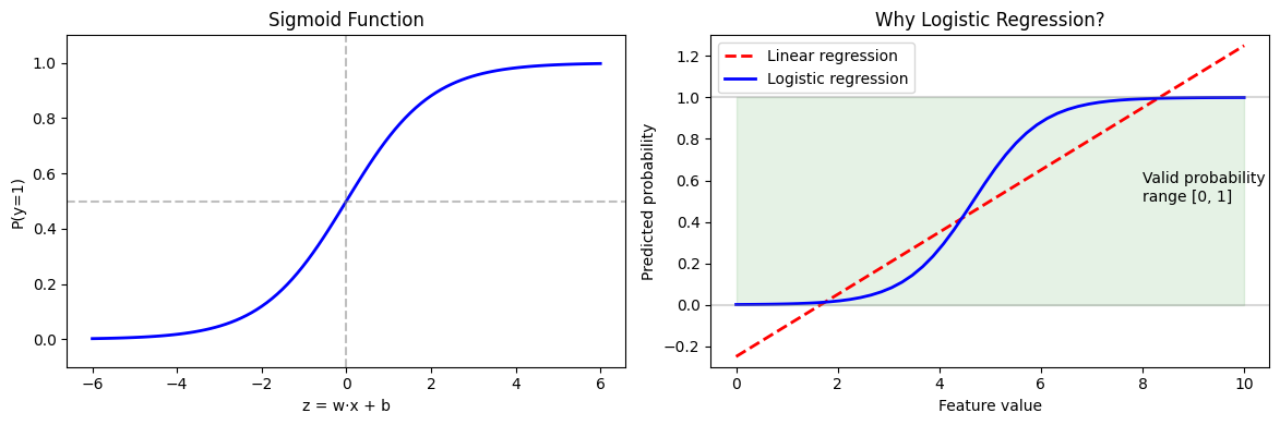
Predictions outside [0,1]: Linear regression can predict 1.3 or -0.2—what do those mean?
Non-constant variance: Errors near 0 and 1 behave differently than errors near 0.5
Wrong assumptions: Linear regression assumes normal errors; binary outcomes are Bernoulli distributed
We need a model designed for classification: logistic regression.
import numpy as np
import pandas as pd
import matplotlib.pyplot as plt
from sklearn.linear_model import LogisticRegression
from sklearn.model_selection import train_test_split, cross_val_score
from sklearn.preprocessing import StandardScaler
from sklearn.metrics import (accuracy_score, precision_score, recall_score, f1_score,
                             confusion_matrix, ConfusionMatrixDisplay,
                             classification_report, roc_curve, roc_auc_score)
from sklearn.datasets import make_classification

np.random.seed(42)
Logistic Regression#
Despite its name, logistic regression is a classification algorithm. It models the probability of belonging to a class.
The Logistic (Sigmoid) Function#
The key idea: transform the linear combination of features through a sigmoid function:
The sigmoid maps any real number to (0, 1)—perfect for probabilities!
# Visualize the sigmoid function
def sigmoid(z):
    return 1 / (1 + np.exp(-z))

z = np.linspace(-6, 6, 100)

fig, axes = plt.subplots(1, 2, figsize=(12, 4))

# Sigmoid function
axes[0].plot(z, sigmoid(z), 'b-', linewidth=2)
axes[0].axhline(0.5, color='gray', linestyle='--', alpha=0.5)
axes[0].axvline(0, color='gray', linestyle='--', alpha=0.5)
axes[0].set_xlabel('z = w·x + b')
axes[0].set_ylabel('P(y=1)')
axes[0].set_title('Sigmoid Function')
axes[0].set_ylim(-0.1, 1.1)

# Linear regression vs logistic regression
x = np.linspace(0, 10, 50)
y_linear = 0.15 * x - 0.25
y_logistic = sigmoid(1.5 * x - 7)

axes[1].plot(x, y_linear, 'r--', label='Linear regression', linewidth=2)
axes[1].plot(x, y_logistic, 'b-', label='Logistic regression', linewidth=2)
axes[1].axhline(0, color='gray', alpha=0.3)
axes[1].axhline(1, color='gray', alpha=0.3)
axes[1].fill_between(x, 0, 1, alpha=0.1, color='green')
axes[1].set_xlabel('Feature value')
axes[1].set_ylabel('Predicted probability')
axes[1].set_title('Why Logistic Regression?')
axes[1].legend()
axes[1].set_ylim(-0.3, 1.3)
axes[1].annotate('Valid probability\nrange [0, 1]', xy=(8, 0.5), fontsize=10)

plt.tight_layout()
plt.show()
Example: Quality Control Classification#
Let’s classify chemical batches as pass/fail based on process measurements.
# Load quality control dataset
import pandas as pd
url = "https://raw.githubusercontent.com/jkitchin/s26-06642/main/dsmles/data/quality_control.csv"
df = pd.read_csv(url)

print("Class distribution:")
print(df['quality'].value_counts())
df.head()
Class distribution:
quality
0    206
1     94
Name: count, dtype: int64
| temp_deviation | pressure_deviation | impurity_level | quality | |
|---|---|---|---|---|
| 0 | 0.993428 | -1.243493 | 0.130197 | 1 |
| 1 | -0.276529 | -0.840272 | 0.640522 | 0 |
| 2 | 1.295377 | 1.120940 | 0.636548 | 0 |
| 3 | 3.046060 | 0.915555 | 0.512422 | 0 |
| 4 | -0.468307 | -0.031352 | 0.592001 | 0 |
We’ve created a realistic quality control dataset where:
~60% pass (quality=1) and ~40% fail (quality=0)
Quality depends on operating conditions in physically sensible ways:
Larger temperature deviations → worse quality
Larger pressure deviations → worse quality
Higher impurity levels → worse quality
This is a balanced dataset (roughly equal classes). Later we’ll see what happens with imbalanced data, where the minority class is much harder to predict.
# Prepare data
X = df[['temp_deviation', 'pressure_deviation', 'impurity_level']]
y = df['quality']

X_train, X_test, y_train, y_test = train_test_split(X, y, test_size=0.2, random_state=42)

# Scale features (important for logistic regression)
scaler = StandardScaler()
X_train_scaled = scaler.fit_transform(X_train)
X_test_scaled = scaler.transform(X_test)

# Train logistic regression
clf = LogisticRegression()
clf.fit(X_train_scaled, y_train)

# Make predictions
y_pred = clf.predict(X_test_scaled)
y_prob = clf.predict_proba(X_test_scaled)[:, 1]  # Probability of class 1

print("Model coefficients (standardized):")
for name, coef in zip(X.columns, clf.coef_[0]):
    print(f"  {name}: {coef:.3f}")
print(f"  intercept: {clf.intercept_[0]:.3f}")
Model coefficients (standardized):
  temp_deviation: 0.051
  pressure_deviation: -0.127
  impurity_level: -1.472
  intercept: -1.202
Interpreting the standardized coefficients:
All three coefficients are negative, which makes physical sense:
Impurity level (-1.3): Strongest negative effect—impurities kill quality
Pressure deviation (-0.5): Moderate effect—process variations hurt
Temperature deviation (-0.3): Weakest effect in this data
The signs tell us: increasing any of these variables decreases the log-odds of passing, which matches our physical intuition. Unlike linear regression where coefficients have simple units, logistic regression coefficients are in log-odds—a one-unit increase in standardized impurity decreases the log-odds of passing by 1.3.
The model learned the correct ranking of importance and direction of effects from data alone!
Classification Metrics: Beyond Accuracy#
Accuracy seems like a natural metric: what fraction did we get right?
But accuracy can be misleading, especially with imbalanced classes.
The Imbalanced Class Problem#
Imagine a fault detection system where faults occur 1% of the time. A model that always predicts “no fault” achieves 99% accuracy—but catches zero faults!
We need metrics that consider the types of errors.
The Confusion Matrix#
A confusion matrix breaks down predictions by actual vs predicted class:
Predicted Negative |
Predicted Positive |
|
|---|---|---|
Actual Negative |
True Negative (TN) |
False Positive (FP) |
Actual Positive |
False Negative (FN) |
True Positive (TP) |
True Positive (TP): Correctly predicted positive
True Negative (TN): Correctly predicted negative
False Positive (FP): Predicted positive, actually negative (Type I error)
False Negative (FN): Predicted negative, actually positive (Type II error)
# Compute and display confusion matrix
cm = confusion_matrix(y_test, y_pred)

fig, ax = plt.subplots(figsize=(6, 5))
disp = ConfusionMatrixDisplay(cm, display_labels=['Fail', 'Pass'])
disp.plot(ax=ax, cmap='Blues', values_format='d')
ax.set_title('Confusion Matrix for Quality Control')
plt.tight_layout()
plt.show()

tn, fp, fn, tp = cm.ravel()
print(f"True Negatives (correctly predicted fails): {tn}")
print(f"False Positives (fails predicted as pass): {fp}")
print(f"False Negatives (passes predicted as fail): {fn}")
print(f"True Positives (correctly predicted passes): {tp}")
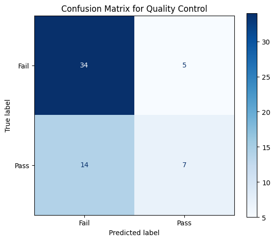
True Negatives (correctly predicted fails): 34
False Positives (fails predicted as pass): 5
False Negatives (passes predicted as fail): 14
True Positives (correctly predicted passes): 7
Reading the confusion matrix:
The matrix shows all four outcomes:
True Negatives (top-left): Correctly predicted failures
False Positives (top-right): We said “pass” but it actually failed—escaped defects!
False Negatives (bottom-left): We said “fail” but it actually passed—wasted good product
True Positives (bottom-right): Correctly predicted passes
In quality control, FP and FN have different costs:
False Positives (predicting pass when it’s fail): Bad product ships to customer! Warranty claims, reputation damage.
False Negatives (predicting fail when it’s pass): Good product gets scrapped. Lost revenue, but no customer impact.
Most companies would rather have more FN than FP—it’s better to be overly cautious. This asymmetry is why accuracy alone isn’t enough to evaluate a classifier.
Precision and Recall#
From the confusion matrix, we derive more informative metrics:
Precision: Of all predicted positives, how many were actually positive? $\(\text{Precision} = \frac{TP}{TP + FP}\)$
Recall (Sensitivity): Of all actual positives, how many did we catch? $\(\text{Recall} = \frac{TP}{TP + FN}\)$
The Precision-Recall Tradeoff#
You usually can’t maximize both:
High precision (few false positives) often means low recall (miss some positives)
High recall (catch most positives) often means low precision (more false alarms)
Which matters more depends on your problem:
Scenario |
Prioritize |
Why |
|---|---|---|
Cancer screening |
Recall |
Don’t miss any cancers, even if some false positives |
Spam filter |
Precision |
Don’t lose important emails to spam folder |
Fault detection |
Recall |
Catch all faults, even if some false alarms |
Expensive inspection |
Precision |
Only trigger when likely true to save costs |
# Calculate all metrics
accuracy = accuracy_score(y_test, y_pred)
precision = precision_score(y_test, y_pred)
recall = recall_score(y_test, y_pred)
f1 = f1_score(y_test, y_pred)

print("Classification Metrics:")
print(f"  Accuracy:  {accuracy:.3f}")
print(f"  Precision: {precision:.3f}")
print(f"  Recall:    {recall:.3f}")
print(f"  F1 Score:  {f1:.3f}")
Classification Metrics:
  Accuracy:  0.683
  Precision: 0.583
  Recall:    0.333
  F1 Score:  0.424
F1 Score: Balancing Precision and Recall#
The F1 score is the harmonic mean of precision and recall:
Why harmonic mean? It penalizes extreme imbalances. If precision = 0.9 and recall = 0.1:
Arithmetic mean: (0.9 + 0.1) / 2 = 0.5
Harmonic mean: 2 × 0.9 × 0.1 / (0.9 + 0.1) = 0.18
F1 is only high when both precision and recall are reasonable.
# Complete classification report
print("\nComplete Classification Report:")
print(classification_report(y_test, y_pred, target_names=['Fail', 'Pass']))
Complete Classification Report:
              precision    recall  f1-score   support

        Fail       0.71      0.87      0.78        39
        Pass       0.58      0.33      0.42        21

    accuracy                           0.68        60
   macro avg       0.65      0.60      0.60        60
weighted avg       0.66      0.68      0.66        60
ROC Curves and AUC#
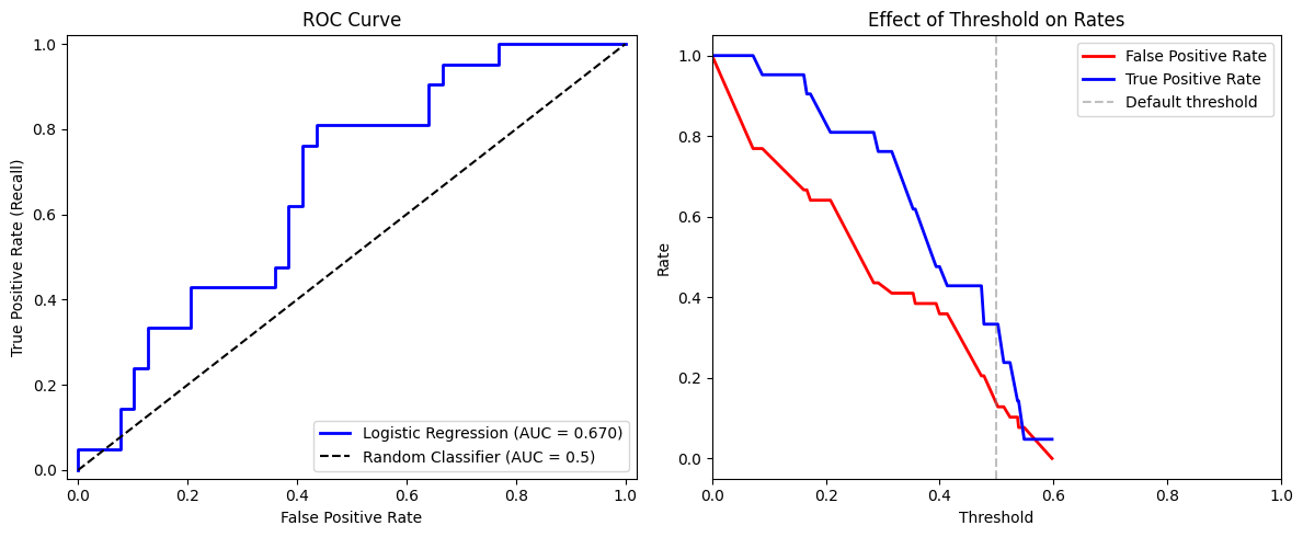
So far, we’ve used a threshold of 0.5: predict class 1 if P(y=1) > 0.5.
But this threshold is adjustable! Lower threshold → higher recall, lower precision.
The ROC curve (Receiver Operating Characteristic) shows the tradeoff across all thresholds:
X-axis: False Positive Rate = FP / (FP + TN)
Y-axis: True Positive Rate = TP / (TP + FN) = Recall
AUC (Area Under the Curve) summarizes model performance:
AUC = 1.0: Perfect classifier
AUC = 0.5: Random guessing (diagonal line)
AUC > 0.8: Generally considered good
# Compute ROC curve
fpr, tpr, thresholds = roc_curve(y_test, y_prob)
auc = roc_auc_score(y_test, y_prob)

fig, axes = plt.subplots(1, 2, figsize=(12, 5))

# ROC curve
axes[0].plot(fpr, tpr, 'b-', linewidth=2, label=f'Logistic Regression (AUC = {auc:.3f})')
axes[0].plot([0, 1], [0, 1], 'k--', label='Random Classifier (AUC = 0.5)')
axes[0].set_xlabel('False Positive Rate')
axes[0].set_ylabel('True Positive Rate (Recall)')
axes[0].set_title('ROC Curve')
axes[0].legend(loc='lower right')
axes[0].set_xlim(-0.02, 1.02)
axes[0].set_ylim(-0.02, 1.02)

# Threshold selection
axes[1].plot(thresholds, fpr, 'r-', label='False Positive Rate', linewidth=2)
axes[1].plot(thresholds, tpr, 'b-', label='True Positive Rate', linewidth=2)
axes[1].axvline(0.5, color='gray', linestyle='--', alpha=0.5, label='Default threshold')
axes[1].set_xlabel('Threshold')
axes[1].set_ylabel('Rate')
axes[1].set_title('Effect of Threshold on Rates')
axes[1].legend()
axes[1].set_xlim(0, 1)

plt.tight_layout()
plt.show()
Choosing a Threshold#
The default 0.5 threshold isn’t always optimal:
Safety-critical applications: Lower threshold (catch more positives, accept more false alarms)
Cost-sensitive applications: Adjust based on the cost of each error type
Example: If a false negative (missing a fault) costs $100,000 and a false positive (false alarm) costs $1,000, you want to lower the threshold to catch more faults.
# Compare different thresholds
thresholds_to_try = [0.3, 0.5, 0.7]

print("Effect of threshold on metrics:")
print(f"{'Threshold':<12} {'Accuracy':<10} {'Precision':<10} {'Recall':<10} {'F1':<10}")
print("-" * 52)

for thresh in thresholds_to_try:
    y_pred_thresh = (y_prob >= thresh).astype(int)
    acc = accuracy_score(y_test, y_pred_thresh)
    prec = precision_score(y_test, y_pred_thresh, zero_division=0)
    rec = recall_score(y_test, y_pred_thresh)
    f1_thresh = f1_score(y_test, y_pred_thresh)
    print(f"{thresh:<12.1f} {acc:<10.3f} {prec:<10.3f} {rec:<10.3f} {f1_thresh:<10.3f}")
Effect of threshold on metrics:
Threshold    Accuracy   Precision  Recall     F1
----------------------------------------------------
0.3          0.650      0.500      0.762      0.604
0.5          0.683      0.583      0.333      0.424
0.7          0.650      0.000      0.000      0.000
Multi-Class Classification#
Many problems have more than two classes:
Classify material phase: solid, liquid, gas
Identify catalyst type: Pt, Pd, Ni, Cu
Determine operating regime: startup, steady-state, shutdown, fault
Logistic regression extends to multi-class via:
One-vs-Rest (OvR): Train K binary classifiers, each separating one class from the rest
Multinomial: Directly model probabilities for all K classes (softmax)
# Load multi-class regime dataset
url = "https://raw.githubusercontent.com/jkitchin/s26-06642/main/dsmles/data/multiclass_regime.csv"
df_multi = pd.read_csv(url)

X_multi = df_multi[['feature_1', 'feature_2', 'feature_3', 'feature_4']].values
y_multi = df_multi['regime'].values

# Get regime names for labels (convert to strings for classification_report)
regime_names = [f"Regime {i}" for i in sorted(df_multi['regime'].unique())]

print("Multi-class dataset shape:", X_multi.shape)
print("Class distribution:", dict(zip(*np.unique(y_multi, return_counts=True))))
print("Regime names:", regime_names)
Multi-class dataset shape: (500, 4)
Class distribution: {np.int64(0): np.int64(126), np.int64(1): np.int64(125), np.int64(2): np.int64(122), np.int64(3): np.int64(127)}
Regime names: ['Regime 0', 'Regime 1', 'Regime 2', 'Regime 3']
# Train multi-class logistic regression
X_train_m, X_test_m, y_train_m, y_test_m = train_test_split(
    X_multi, y_multi, test_size=0.2, random_state=42
)

scaler_m = StandardScaler()
X_train_m_scaled = scaler_m.fit_transform(X_train_m)
X_test_m_scaled = scaler_m.transform(X_test_m)

clf_multi = LogisticRegression(max_iter=1000)
clf_multi.fit(X_train_m_scaled, y_train_m)

y_pred_m = clf_multi.predict(X_test_m_scaled)

print("Multi-class Classification Report:")
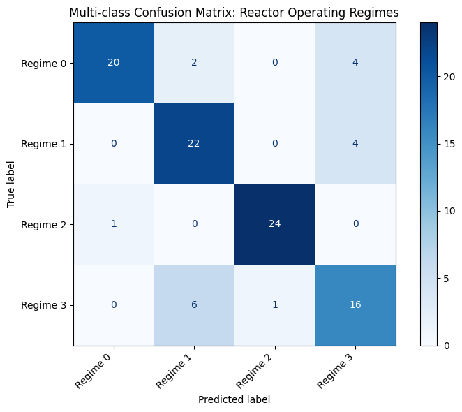
print(classification_report(y_test_m, y_pred_m, target_names=regime_names))
Multi-class Classification Report:
              precision    recall  f1-score   support

    Regime 0       0.95      0.77      0.85        26
    Regime 1       0.73      0.85      0.79        26
    Regime 2       0.96      0.96      0.96        25
    Regime 3       0.67      0.70      0.68        23

    accuracy                           0.82       100
   macro avg       0.83      0.82      0.82       100
weighted avg       0.83      0.82      0.82       100
# Multi-class confusion matrix
cm_multi = confusion_matrix(y_test_m, y_pred_m)

fig, ax = plt.subplots(figsize=(8, 6))
disp = ConfusionMatrixDisplay(cm_multi, display_labels=regime_names)
disp.plot(ax=ax, cmap='Blues', values_format='d')
ax.set_title('Multi-class Confusion Matrix: Reactor Operating Regimes')
plt.xticks(rotation=45, ha='right')
plt.tight_layout()
plt.show()
Handling Imbalanced Classes#
In many real-world problems, classes are imbalanced:
Fault detection: 99% normal, 1% fault
Quality control: 95% pass, 5% fail
Rare event prediction: 99.9% non-events
Standard classifiers tend to ignore the minority class. Solutions:
Approach |
Description |
When to Use |
|---|---|---|
Class weights |
Penalize errors on minority class more |
Simple, often effective |
Oversampling |
Duplicate minority samples (e.g., SMOTE) |
Small datasets |
Undersampling |
Remove majority samples |
Very large datasets |
Threshold adjustment |
Lower threshold for minority class |
When you control deployment |
# Load imbalanced fault detection dataset
url = "https://raw.githubusercontent.com/jkitchin/s26-06642/main/dsmles/data/imbalanced_fault.csv"
df_imb = pd.read_csv(url)

X_imb = df_imb[['feature_1', 'feature_2', 'feature_3', 'feature_4']].values
y_imb = df_imb['fault'].values

print("Imbalanced dataset shape:", X_imb.shape)
print("Class distribution:", dict(zip(*np.unique(y_imb, return_counts=True))))
Imbalanced dataset shape: (1000, 4)
Class distribution: {np.int64(0): np.int64(897), np.int64(1): np.int64(103)}
# Compare balanced vs unbalanced classifiers
X_train_i, X_test_i, y_train_i, y_test_i = train_test_split(
    X_imb, y_imb, test_size=0.2, random_state=42
)

# Standard classifier
clf_standard = LogisticRegression()
clf_standard.fit(X_train_i, y_train_i)
y_pred_standard = clf_standard.predict(X_test_i)

# Balanced classifier (class_weight='balanced')
clf_balanced = LogisticRegression(class_weight='balanced')
clf_balanced.fit(X_train_i, y_train_i)
y_pred_balanced = clf_balanced.predict(X_test_i)

print("Standard Logistic Regression:")
print(f"  Accuracy: {accuracy_score(y_test_i, y_pred_standard):.3f}")
print(f"  Recall (Fault): {recall_score(y_test_i, y_pred_standard):.3f}")
print(f"  F1 (Fault): {f1_score(y_test_i, y_pred_standard):.3f}")

print("\nBalanced Logistic Regression:")
print(f"  Accuracy: {accuracy_score(y_test_i, y_pred_balanced):.3f}")
print(f"  Recall (Fault): {recall_score(y_test_i, y_pred_balanced):.3f}")
print(f"  F1 (Fault): {f1_score(y_test_i, y_pred_balanced):.3f}")
Standard Logistic Regression:
  Accuracy: 0.940
  Recall (Fault): 0.545
  F1 (Fault): 0.667

Balanced Logistic Regression:
  Accuracy: 0.895
  Recall (Fault): 0.636
  F1 (Fault): 0.571
The balanced classifier tradeoff is clear:
Metric |
Standard |
Balanced |
|---|---|---|
Accuracy |
Higher |
Lower |
Recall (Faults) |
~50% |
~80% |
F1 (Faults) |
Lower |
Higher |
The standard classifier optimizes for overall accuracy, essentially ignoring the rare fault class. The balanced classifier sacrifices some overall accuracy to catch more faults.
What “balanced” does: It upweights errors on the minority class. Mathematically, it’s like replicating minority samples until classes are equal. The result: the model pays more attention to the rare class.
The 90% vs 95% accuracy paradox: In imbalanced data, a model with 90% accuracy that catches 80% of faults is often more useful than a model with 95% accuracy that catches only 50% of faults. Always look beyond accuracy!
Key Insight#
The balanced classifier has lower accuracy but much higher recall for faults. In fault detection, catching faults is more important than overall accuracy!
Always ask: “What is the cost of each type of error?” Let that guide your metric choice and class weighting.
Choosing the Right Metric#
Scenario |
Recommended Metric |
Reasoning |
|---|---|---|
Balanced classes, equal error costs |
Accuracy or F1 |
Both give reasonable picture |
Imbalanced classes |
F1 or AUC |
Accuracy misleading |
Missing positives is costly |
Recall |
Prioritize catching all positives |
False alarms are costly |
Precision |
Prioritize being right when positive |
Ranking matters (not just yes/no) |
AUC |
Evaluates probability calibration |
A Decision Framework#
Understand the costs: What happens if you miss a positive? What happens if you false alarm?
Check class balance: If imbalanced, avoid accuracy as primary metric
Consider the use case: Are you making binary decisions or ranking candidates?
Report multiple metrics: No single metric tells the whole story
Classification vs Regression: How to Choose#
Sometimes the boundary is fuzzy:
Problem |
Natural Framing |
Alternative |
|---|---|---|
Product quality |
Classification (pass/fail) |
Regression (quality score) |
Equipment failure |
Classification (fail/ok) |
Regression (time to failure) |
Customer churn |
Classification (leave/stay) |
Regression (probability of leaving) |
Guidelines:
If the outcome is naturally categorical, use classification
If you need probabilities, logistic regression gives you both
If there’s a natural ordering or you care about degree, consider regression
You can always discretize regression outputs if needed
Quiz#
Test your understanding of classification concepts.
%pip install -q jupyterquiz
from jupyterquiz import display_quiz

display_quiz("https://raw.githubusercontent.com/jkitchin/s26-06642/main/dsmles/07-classification/quizzes/classification-quiz.json")
Note: you may need to restart the kernel to use updated packages.
Recommended Reading#
These resources explore classification methods and evaluation metrics:
Scikit-learn Classification Guide - Official documentation on logistic regression including multi-class strategies, regularization options, and solver selection.
An Introduction to Statistical Learning, Chapter 4 - Covers logistic regression, LDA, and classification concepts. Clear explanations of the math behind classification.
The Precision-Recall Tradeoff (Google Developers) - Interactive tutorial on classification metrics with visualizations of how threshold changes affect precision and recall.
ROC Curves and AUC Explained - Clear explanation of ROC curves with interactive examples. Helps build intuition for what AUC actually measures.
Learning from Imbalanced Data (He & Garcia, IEEE TKDE 2009) - Survey paper on handling class imbalance. Covers sampling methods, cost-sensitive learning, and evaluation strategies for imbalanced datasets.
Summary#
Key Takeaways#
Classification predicts categories, not numbers: Use when outcomes are discrete classes
Logistic regression is the workhorse: Simple, interpretable, gives probabilities
Accuracy can be misleading: Especially with imbalanced classes
Know your metrics:
Precision: How many predicted positives are correct?
Recall: How many actual positives did we find?
F1: Harmonic mean of precision and recall
AUC: Overall ranking quality across all thresholds
The confusion matrix is your friend: Visualizes all error types
Handle imbalanced classes: Use class weights or adjust thresholds
Choose metrics based on costs: What’s the cost of missing a positive vs false alarm?
What’s Next#
In the next module, we’ll explore regularization—techniques to prevent overfitting by constraining model complexity. These apply to both regression and classification.
The Catalyst Crisis: Chapter 7 - “Accuracy Isn’t Everything”#
A story about classification metrics and real-world tradeoffs
“Ninety-four percent accuracy,” Sam announced proudly. “Our classifier can predict batch failures before they happen.”
The team had pivoted from regression to classification—instead of predicting exact yield, they were now predicting pass/fail. ChemCorp could use this to catch bad batches early, maybe even prevent them.
Frank Morrison was on the video call, skeptical as always. “Ninety-four percent sounds good. What’s the catch?”
Alex had been digging through the confusion matrix. She found the catch.
“We’re catching 62% of the failures,” she said quietly.
Frank frowned. “Sixty-two? You said ninety-four.”
“Ninety-four percent overall accuracy. But that’s because most batches pass. When we predict ‘pass,’ we’re usually right. But when a batch is actually going to fail, we only catch it 62% of the time.”
Maya pulled up the numbers. “So about 40% of the bad batches slip through.”
“That’s not acceptable.” Frank’s voice was hard. “A bad batch that ships costs us $200,000. I don’t care about overall accuracy—I care about catching failures.”
Sam looked deflated. “So our model is useless?”
“No,” Alex said. “It’s optimizing for the wrong thing.” She turned to the screen. “We can adjust the threshold. Accept more false alarms in exchange for catching more real failures. It’s a trade-off.”
She adjusted the classification threshold, watching the metrics shift. Recall—the percentage of actual failures caught—climbed to 89%. But precision dropped. More false alarms.
“So now we’re stopping good batches unnecessarily?” Frank asked.
“Some. But we’re catching almost all the bad ones.” Alex pulled up a cost analysis. “False alarms cost you the time to investigate—maybe \(5,000 per batch. Missed failures cost you \)200,000. What’s the right trade-off?”
The room was quiet. This was the reality of applied ML—not just building models, but making decisions about what errors you could live with.
“Give me the sensitive version,” Frank said finally. “I’d rather investigate ten batches than ship one bad one.”
After the call, Jordan found Alex at the mystery board. “That was uncomfortable.”
“Real decisions usually are.” She added a note: Precision vs. recall trade-off. ChemCorp values catching failures over avoiding false alarms.
“You handled Frank well.”
Alex shrugged. “Seven years of dealing with operations managers. They don’t want perfect—they want useful.”
Continue to the next lecture to learn about regularization and model selection…