Module 03: Intermediate Pandas

Advanced data manipulation techniques for real-world data analysis.

Learning Objectives

1. Use groupby for split-apply-combine operations

2. Merge and join DataFrames

3. Reshape data with pivot and melt

4. Apply custom functions efficiently

5. Work with datetime data

import pandas as pd
import numpy as np
import matplotlib.pyplot as plt

# Load experiments dataset
import pandas as pd

url = "https://raw.githubusercontent.com/jkitchin/s26-06642/main/dsmles/data/experiments_intermediate.csv"
experiments = pd.read_csv(url, parse_dates=['date'])

print(f"Dataset shape: {experiments.shape}")
experiments.head()

Dataset shape: (50, 8)

	experiment_id	date	catalyst	temperature	pressure	conversion	selectivity	yield
0	EXP001	2024-01-01	Ru/Al2O3	350	4.1	0.832	0.893	74.3
1	EXP002	2024-01-02	Pt/Al2O3	300	1.3	0.859	0.808	69.4
2	EXP003	2024-01-03	Ru/Al2O3	350	2.4	0.305	0.962	29.3
3	EXP004	2024-01-04	Ru/Al2O3	500	1.5	0.632	0.739	46.7
4	EXP005	2024-01-05	Pt/Al2O3	350	4.5	0.571	0.795	45.4

GroupBy: The Split-Apply-Combine Pattern

GroupBy is arguably the most powerful Pandas operation. It lets you answer questions like:

• “What’s the average yield for each catalyst?”

• “What’s the best-performing temperature for each reactor?”

• “How does conversion vary by day of week?”

The Mental Model: Split-Apply-Combine

1. Split: Divide data into groups based on one or more columns

2. Apply: Perform some operation on each group

3. Combine: Combine results back into a DataFrame

This is the Pandas equivalent of SQL’s GROUP BY, but more flexible.

When to Use GroupBy

• Comparing performance across categories (catalysts, reactors, operators)

• Aggregating replicate experiments

• Computing statistics within subgroups

• Normalizing data within groups

# Basic groupby: mean by catalyst
experiments.groupby('catalyst')['yield'].mean()

catalyst
Pd/Al2O3    46.633333
Pt/Al2O3    49.206667
Ru/Al2O3    52.880000
Name: yield, dtype: float64

# Multiple aggregations
experiments.groupby('catalyst')['yield'].agg(['mean', 'std', 'min', 'max', 'count'])

	mean	std	min	max	count
catalyst
Pd/Al2O3	46.633333	12.843490	25.9	67.2	15
Pt/Al2O3	49.206667	15.956703	29.4	78.3	15
Ru/Al2O3	52.880000	17.198519	26.7	81.9	20

# Group by multiple columns
experiments.groupby(['catalyst', 'temperature'])['yield'].mean().unstack()

temperature	300	350	400	450	500
catalyst
Pd/Al2O3	31.80	40.250000	44.466667	56.200000	46.15
Pt/Al2O3	47.84	50.766667	NaN	52.383333	32.30
Ru/Al2O3	45.30	55.540000	42.950000	50.933333	60.00

# Different aggregations for different columns
experiments.groupby('catalyst').agg({
    'conversion': 'mean',
    'selectivity': 'mean',
    'yield': ['mean', 'std'],
    'experiment_id': 'count'
})

	conversion	selectivity	yield		experiment_id
	mean	mean	mean	std	count
catalyst
Pd/Al2O3	0.575133	0.819733	46.633333	12.843490	15
Pt/Al2O3	0.578400	0.843467	49.206667	15.956703	15
Ru/Al2O3	0.625400	0.854450	52.880000	17.198519	20

# Named aggregations (cleaner column names)
summary = experiments.groupby('catalyst').agg(
    n_experiments=('experiment_id', 'count'),
    mean_yield=('yield', 'mean'),
    std_yield=('yield', 'std'),
    max_yield=('yield', 'max')
).round(2)

summary

	n_experiments	mean_yield	std_yield	max_yield
catalyst
Pd/Al2O3	15	46.63	12.84	67.2
Pt/Al2O3	15	49.21	15.96	78.3
Ru/Al2O3	20	52.88	17.20	81.9

# Custom aggregation function
def yield_range(x):
    return x.max() - x.min()

experiments.groupby('catalyst')['yield'].agg(['mean', yield_range])

	mean	yield_range
catalyst
Pd/Al2O3	46.633333	41.3
Pt/Al2O3	49.206667	48.9
Ru/Al2O3	52.880000	55.2

Merging DataFrames: Combining Data Sources

Real analysis often requires combining data from multiple sources:

• Experiment results + catalyst properties

• Sensor readings + equipment specifications

• Lab data + literature values

The Four Types of Merges

Type	What It Keeps	Use When
inner	Only matching rows	You only want complete records
left	All rows from left table	Your main table is on the left, reference data on right
right	All rows from right table	Your main table is on the right
outer	All rows from both	You want to see what’s missing

The Key Concept: Join Keys

The on parameter specifies which column(s) to match. Make sure:

• The columns have the same meaning in both tables

• Values are comparable (watch out for “Pt” vs “Pt/Al2O3”)

• Missing keys are handled appropriately (check for NaN after merge)

# Load catalyst properties reference table
url = "https://raw.githubusercontent.com/jkitchin/s26-06642/main/dsmles/data/catalyst_info.csv"
catalyst_info = pd.read_csv(url)
catalyst_info

	catalyst	metal_loading	surface_area	cost_per_kg
0	Pt/Al2O3	1.0	250	50000
1	Pd/Al2O3	0.5	280	30000
2	Ru/Al2O3	2.0	220	8000
3	Rh/Al2O3	0.3	300	80000

# Merge experiments with catalyst info
merged = experiments.merge(catalyst_info, on='catalyst', how='left')
merged.head()

	experiment_id	date	catalyst	temperature	pressure	conversion	selectivity	yield	metal_loading	surface_area	cost_per_kg
0	EXP001	2024-01-01	Ru/Al2O3	350	4.1	0.832	0.893	74.3	2.0	220	8000
1	EXP002	2024-01-02	Pt/Al2O3	300	1.3	0.859	0.808	69.4	1.0	250	50000
2	EXP003	2024-01-03	Ru/Al2O3	350	2.4	0.305	0.962	29.3	2.0	220	8000
3	EXP004	2024-01-04	Ru/Al2O3	500	1.5	0.632	0.739	46.7	2.0	220	8000
4	EXP005	2024-01-05	Pt/Al2O3	350	4.5	0.571	0.795	45.4	1.0	250	50000

# Different merge types
# how='left'   - Keep all rows from left DataFrame
# how='right'  - Keep all rows from right DataFrame
# how='inner'  - Keep only matching rows (intersection)
# how='outer'  - Keep all rows from both (union)

# Example: inner merge (Rh/Al2O3 exists in catalyst_info but not in experiments)
inner_merge = experiments.merge(catalyst_info, on='catalyst', how='inner')
print(f"Left: {len(experiments)}, Right: {len(catalyst_info)}, Inner: {len(inner_merge)}")

Left: 50, Right: 4, Inner: 50

Reshaping Data: Pivot and Melt

Data comes in different “shapes,” and sometimes you need to reshape it:

Long vs Wide Format

Long format (tidy data):

• Each row is one observation

• Good for analysis and plotting

• Example: Each row = (catalyst, temperature, yield)

Wide format (spreadsheet-style):

• Columns represent different conditions

• Easier for humans to read

• Example: Rows = catalysts, Columns = temperatures, Values = yields

When to Use Which

Format	Use For
Long	Most Pandas operations, plotting, ML
Wide	Display tables, Excel export, certain visualizations

The Transformation Tools

• pivot_table(): Long → Wide (aggregate if needed)

• melt(): Wide → Long (unpivot)

# Pivot: long to wide format
# Create summary table: catalysts as rows, temperatures as columns
pivot_table = experiments.pivot_table(
    values='yield',
    index='catalyst',
    columns='temperature',
    aggfunc='mean'
).round(1)

pivot_table

temperature	300	350	400	450	500
catalyst
Pd/Al2O3	31.8	40.2	44.5	56.2	46.2
Pt/Al2O3	47.8	50.8	NaN	52.4	32.3
Ru/Al2O3	45.3	55.5	43.0	50.9	60.0

# Multiple values in pivot
pivot_multi = experiments.pivot_table(
    values=['conversion', 'selectivity'],
    index='catalyst',
    columns='temperature',
    aggfunc='mean'
).round(2)

pivot_multi

	conversion					selectivity
temperature	300	350	400	450	500	300	350	400	450	500
catalyst
Pd/Al2O3	0.45	0.44	0.59	0.68	0.61	0.70	0.90	0.76	0.84	0.76
Pt/Al2O3	0.58	0.58	NaN	0.62	0.36	0.82	0.88	NaN	0.84	0.90
Ru/Al2O3	0.54	0.66	0.47	0.61	0.71	0.85	0.84	0.89	0.86	0.85

# Melt: wide to long format
# Useful when data is in "spreadsheet" format
wide_data = pd.DataFrame({
    'catalyst': ['Pt', 'Pd', 'Ru'],
    'yield_300K': [45, 42, 38],
    'yield_400K': [65, 62, 55],
    'yield_500K': [78, 75, 68]
})

print("Wide format:")
print(wide_data)

# Convert to long format
long_data = wide_data.melt(
    id_vars='catalyst',
    var_name='condition',
    value_name='yield'
)

print("\nLong format:")
print(long_data)

Wide format:
  catalyst  yield_300K  yield_400K  yield_500K
0       Pt          45          65          78
1       Pd          42          62          75
2       Ru          38          55          68

Long format:
  catalyst   condition  yield
0       Pt  yield_300K     45
1       Pd  yield_300K     42
2       Ru  yield_300K     38
3       Pt  yield_400K     65
4       Pd  yield_400K     62
5       Ru  yield_400K     55
6       Pt  yield_500K     78
7       Pd  yield_500K     75
8       Ru  yield_500K     68

Apply and Transform

# Apply a function to each row
def categorize_yield(row):
    if row['yield'] >= 70:
        return 'high'
    elif row['yield'] >= 50:
        return 'medium'
    else:
        return 'low'

experiments['yield_category'] = experiments.apply(categorize_yield, axis=1)
experiments[['experiment_id', 'yield', 'yield_category']].head(10)

	experiment_id	yield	yield_category
0	EXP001	74.3	high
1	EXP002	69.4	medium
2	EXP003	29.3	low
3	EXP004	46.7	low
4	EXP005	45.4	low
5	EXP006	32.5	low
6	EXP007	36.3	low
7	EXP008	49.1	low
8	EXP009	70.5	high
9	EXP010	45.1	low

# Transform: apply function but keep original shape
# Useful for normalization within groups

# Z-score normalization of yield within each catalyst group
experiments['yield_zscore'] = experiments.groupby('catalyst')['yield'].transform(
    lambda x: (x - x.mean()) / x.std()
)

experiments[['experiment_id', 'catalyst', 'yield', 'yield_zscore']].head(10)

	experiment_id	catalyst	yield	yield_zscore
0	EXP001	Ru/Al2O3	74.3	1.245456
1	EXP002	Pt/Al2O3	69.4	1.265508
2	EXP003	Ru/Al2O3	29.3	-1.371048
3	EXP004	Ru/Al2O3	46.7	-0.359333
4	EXP005	Pt/Al2O3	45.4	-0.238562
5	EXP006	Pt/Al2O3	32.5	-1.047000
6	EXP007	Ru/Al2O3	36.3	-0.964037
7	EXP008	Pd/Al2O3	49.1	0.192056
8	EXP009	Ru/Al2O3	70.5	1.024507
9	EXP010	Ru/Al2O3	45.1	-0.452365

Working with Dates

# Extract date components
experiments['year'] = experiments['date'].dt.year
experiments['month'] = experiments['date'].dt.month
experiments['week'] = experiments['date'].dt.isocalendar().week
experiments['day_of_week'] = experiments['date'].dt.day_name()

experiments[['date', 'year', 'month', 'week', 'day_of_week']].head()

	date	year	month	week	day_of_week
0	2024-01-01	2024	1	1	Monday
1	2024-01-02	2024	1	1	Tuesday
2	2024-01-03	2024	1	1	Wednesday
3	2024-01-04	2024	1	1	Thursday
4	2024-01-05	2024	1	1	Friday

# Group by time period
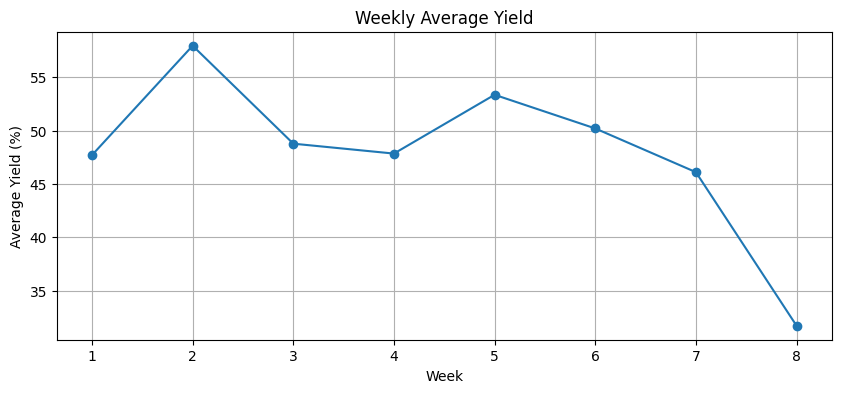
weekly_avg = experiments.groupby('week')['yield'].mean()

plt.figure(figsize=(10, 4))
weekly_avg.plot(kind='line', marker='o')
plt.xlabel('Week')
plt.ylabel('Average Yield (%)')
plt.title('Weekly Average Yield')
plt.grid(True)
plt.show()

# Resample time series data
experiments_ts = experiments.set_index('date')

# Weekly average
weekly = experiments_ts['yield'].resample('W').mean()
print(weekly)

date
2024-01-07    47.700000
2024-01-14    57.957143
2024-01-21    48.771429
2024-01-28    47.842857
2024-02-04    53.357143
2024-02-11    50.200000
2024-02-18    46.100000
2024-02-25    31.700000
Freq: W-SUN, Name: yield, dtype: float64

Method Chaining

Combine operations elegantly.

# Instead of step-by-step:
# df1 = experiments[experiments['temperature'] >= 400]
# df2 = df1.groupby('catalyst')['yield'].mean()
# df3 = df2.sort_values(ascending=False)

# Use method chaining:
result = (
    experiments
    .query('temperature >= 400')  # Filter
    .groupby('catalyst')['yield']  # Group
    .mean()  # Aggregate
    .sort_values(ascending=False)  # Sort
    .round(1)  # Format
)

result

catalyst
Ru/Al2O3    54.4
Pd/Al2O3    50.7
Pt/Al2O3    49.5
Name: yield, dtype: float64

---

The Catalyst Crisis: “The Outlier’s Secret”

Continued from Pandas Introduction…

---

The data point sat alone in the upper right corner of the scatter plot, miles from its companions.

“That’s got to be an error,” Sam said. “Ninety-eight percent yield? The next highest is seventy-two.”

Alex stared at the point. In her years at the refinery, she’d learned to be suspicious of outliers—but not in the way most people meant. Sometimes outliers were errors. Sometimes they were discoveries.

“Can we trace it back?” she asked. “Find the actual batch record?”

Maya pulled up the metadata. “Batch 7,847. March 15th. Night shift.”

“The night of the thunderstorm,” Frank’s voice came through the speaker. He’d been sitting in on their analysis session, mostly silent. “I remember that batch. Power went out for about three minutes. Backup generators kicked in.”

“And you got your best yield ever?”

Frank scratched his chin. “We assumed it was a measurement error. Wrote it off.”

Alex felt a hum of excitement—the feeling she used to get when a process problem suddenly made sense. “What if it wasn’t an error? What if the power outage accidentally created conditions you’d never tried on purpose?”

She pulled up the sensor data from that night. During the three-minute outage, the backup system had run the reflux pump at a higher rate—an unintended consequence of the generator switchover.

“Higher reflux ratio,” Jordan said quietly. “That would change the separation efficiency.”

“By a lot, apparently.” Alex highlighted the data point on the plot. “This isn’t an outlier to remove. It’s an experiment you never meant to run.”

Frank was quiet for a long moment. “We’ve been running this column for twelve years. Same conditions the whole time. You’re telling me a thunderstorm found a better operating point?”

“I’m telling you you should test it intentionally.”

After the meeting, Maya caught Alex by the coffee machine. “How did you know not to delete it?”

Alex poured herself a cup of the questionable brew. “In industry, you learn that the most important data points are usually the weirdest ones. Everyone wants to throw them out because they don’t fit. But they don’t fit because they’re telling you something new.”

She added to the mystery board: Batch 7847: 98% yield during power outage. Higher reflux ratio. Accidental discovery—what else are we missing?

That night, checking her Data Academy profile, she noticed a new badge had appeared: Data Wrangler.

She smiled. Progress.

To be continued…

# Complex analysis in one chain
analysis = (
    experiments
    .assign(yield_category=lambda df: pd.cut(df['yield'], 
                                              bins=[0, 50, 70, 100],
                                              labels=['low', 'medium', 'high']))
    .groupby(['catalyst', 'yield_category'])
    .size()
    .unstack(fill_value=0)
)

analysis

yield_category	low	medium	high
catalyst
Pd/Al2O3	9	6	0
Pt/Al2O3	9	5	1
Ru/Al2O3	10	5	5

Test Your Knowledge

%pip install -q jupyterquiz
from jupyterquiz import display_quiz

display_quiz("https://raw.githubusercontent.com/jkitchin/s26-06642/main/dsmles/03-intermediate-pandas/quizzes/intermediate-pandas-quiz.json")

Note: you may need to restart the kernel to use updated packages.

Recommended Reading

These resources cover advanced Pandas techniques for data transformation:

1. Pandas GroupBy: Your Guide to Grouping Data - An in-depth tutorial on the split-apply-combine pattern with practical examples. Covers aggregation, transformation, and filtration operations.

2. Pandas Merging 101 - A comprehensive Stack Overflow guide covering all types of joins with clear diagrams. Bookmark this for reference when merging DataFrames.

3. Reshaping and Pivot Tables - Official documentation on pivot_table, melt, stack, and unstack. Essential for transforming data between wide and long formats.

4. Modern Pandas (Tom Augspurger) - A blog series on writing idiomatic, efficient Pandas code. Covers method chaining, the pipe method, and performance optimization.

5. Effective Pandas by Matt Harrison - A practical guide to writing clean, efficient Pandas code. Emphasizes modern best practices and method chaining patterns.

Summary: The Data Wrangling Toolkit

Intermediate Pandas is about transforming data to answer complex questions. Here’s your toolkit:

Core Operations

Operation	When to Use	Key Method
GroupBy	Compare across categories	df.groupby('col').agg()
Merge	Combine data sources	df1.merge(df2, on='col')
Pivot	Long → Wide format	df.pivot_table()
Melt	Wide → Long format	df.melt()
Transform	Apply function, keep shape	df.groupby().transform()

The Method Chaining Philosophy

Instead of:

df1 = df[df['temp'] > 400]
df2 = df1.groupby('catalyst')['yield'].mean()
df3 = df2.sort_values(ascending=False)

Write:

(df.query('temp > 400')
   .groupby('catalyst')['yield']
   .mean()
   .sort_values(ascending=False))

Benefits: More readable, fewer intermediate variables, easier to modify.

Key Decisions

Situation	Choice
Need to compare groups?	Use groupby()
Need to combine tables?	Use merge() with appropriate how=
Need to aggregate duplicates?	Use pivot_table(aggfunc=...)
Need to normalize within groups?	Use groupby().transform()

Common Gotchas

• groupby() returns a GroupBy object, not a DataFrame—add .mean(), .agg(), etc.

• merge() may create more rows than expected if keys aren’t unique

• pivot_table() aggregates by default (use aggfunc to control how)

• Watch for column names becoming tuples after complex aggregations

Next Steps

Now that you can manipulate data effectively, we’ll move to dimensionality reduction—techniques for exploring and visualizing high-dimensional datasets before building models.