Optimizing Over Surrogates with MILP

A surrogate model is often fitted so that you can optimize over it: find the operating conditions that minimize cost, or choose equipment inside a larger design problem. If the surrogate is piecewise linear, it can be written into a mixed-integer linear program (MILP) exactly, and a MILP solver then returns the global optimum of the surrogate with a certificate, not just a local one.

JAXSR supports this end to end:

1. BasisLibrary.add_hinges() adds hinge terms \(\max(0, x - k)\) and \(\max(0, k - x)\), which give a MARS-style piecewise-linear fit.

2. milp_incompatible_terms(model) confirms that every selected term has an exact MILP formulation.

3. model.to_pyomo(block) or model.to_discopt(dm_model) writes the fitted model into an optimization model as variables and constraints.

This notebook works through a 1-D example (including an important pitfall and its fix), a 2-D example, a design problem with discrete decisions solved in both Pyomo and discopt, and a catalyst-selection problem with a categorical input. The MIP embedding guide is the reference for the formulations and every option.

Requirements: pip install jaxsr[mip] (Pyomo and HiGHS) and pip install discopt.

import time

import discopt
import matplotlib.pyplot as plt
import numpy as np
import pyomo.environ as pyo

from jaxsr import BasisLibrary, SymbolicRegressor, milp_incompatible_terms

highs = pyo.SolverFactory("appsi_highs")

1. A piecewise-linear fit in 1-D

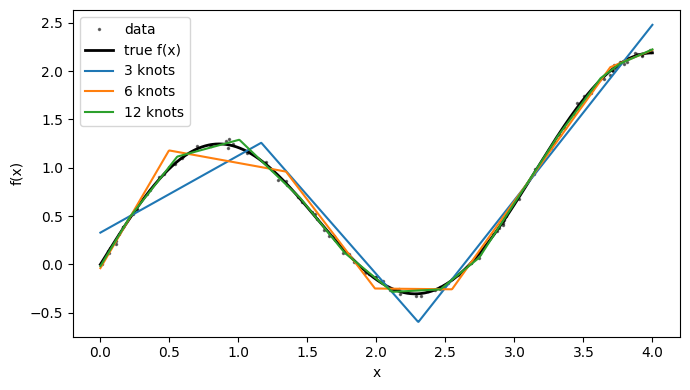
We start with a nonconvex function that has a local minimum at the left edge (\(x = 0\)) and a global minimum near \(x \approx 2.28\):

\[f(x) = \sin(2x) + 0.3x, \qquad x \in [0, 4].\]

We sample it with a little noise, then fit three libraries containing a constant, a linear term and hinges at 3, 6 and 12 knots placed at quantiles of the data. With mirror=True (the default) each knot contributes the pair \(\max(0, x - k)\) and \(\max(0, k - x)\), and BIC decides which hinges are worth keeping.

def f_true(x):
    return np.sin(2 * x) + 0.3 * x


rng = np.random.default_rng(0)
x = rng.uniform(0, 4, 120)
y = f_true(x) + rng.normal(0, 0.02, x.size)
X = x.reshape(-1, 1)


def fit_hinge_model(X, y, n_knots, max_terms=12):
    library = (
        BasisLibrary(n_features=1, feature_names=["x"], feature_bounds=[(0.0, 4.0)])
        .add_constant()
        .add_linear()
        .add_hinges(X=X, n_knots=n_knots)
    )
    model = SymbolicRegressor(
        basis_library=library, max_terms=max_terms, information_criterion="bic"
    )
    return model.fit(X, y)


models = {k: fit_hinge_model(X, y, k) for k in (3, 6, 12)}
for k, model in models.items():
    print(f"{k:2d} knots: {len(model.selected_features_):2d} terms, R2 = {model.metrics_['r2']:.4f}")

 3 knots:  4 terms, R2 = 0.9677
 6 knots:  8 terms, R2 = 0.9921
12 knots: 12 terms, R2 = 0.9991

grid = np.linspace(0, 4, 801)
fig, ax = plt.subplots(figsize=(7, 4))
ax.plot(x, y, "k.", ms=3, alpha=0.5, label="data")
ax.plot(grid, f_true(grid), "k-", lw=2, label="true f(x)")
for k, model in models.items():
    ax.plot(grid, np.asarray(model.predict(grid.reshape(-1, 1))), label=f"{k} knots")
ax.set_xlabel("x")
ax.set_ylabel("f(x)")
ax.legend()
plt.tight_layout()
plt.show()

The fitted expression is an ordinary JAXSR expression, so to_sympy(), to_callable() and save() all work. Before embedding it, we check that every selected term is MILP-representable. An empty list means the embedding is a pure MILP.

model = models[12]
print(model.expression_)
print("non-MILP terms:", milp_incompatible_terms(model))

y = 2.01*max(0,x-2.74485) + 1.093*max(0,2.46303-x) - 1.431*max(0,0.557208-x) - 0.9646*max(0,2.74485-x) - 0.8621*max(0,x-3.62335) - 1.757*max(0,1.00688-x) + 1.241*max(0,2.11603-x) + 0.5945*max(0,x-1.76882) - 0.394*max(0,x-1.44919) - 0.5631*max(0,0.212114-x) - 0.275*max(0,x-3.31162) - 0.4449*max(0,x-3.76412)
non-MILP terms: []

2. Embedding in Pyomo and minimizing

model.to_pyomo() returns a Pyomo ConcreteModel (or fills a Block you pass in). The input and output variables are available as jaxsr_inputs and jaxsr_output. Each hinge whose knot lies inside the input bounds becomes one continuous variable, one binary and four linear constraints (big-M), with the big-M constants computed from the bounds.

def minimize_pyomo(model, **kwargs):
    blk = model.to_pyomo(**kwargs)
    blk.obj = pyo.Objective(expr=blk.jaxsr_output, sense=pyo.minimize)
    highs.solve(blk)
    x_opt = {name: pyo.value(v) for name, v in blk.jaxsr_inputs.items()}
    return x_opt, pyo.value(blk.obj), blk


print(f"{'knots':>5} {'x*':>8} {'surrogate f(x*)':>16} {'true f(x*)':>11} {'binaries':>9}")
for k, m in models.items():
    x_opt, f_opt, blk = minimize_pyomo(m)
    print(f"{k:5d} {x_opt['x']:8.4f} {f_opt:16.4f} {f_true(x_opt['x']):11.4f} {len(blk.binaries):9d}")

x_best = grid[np.argmin(f_true(grid))]
print(f"\ntrue minimum: x = {x_best:.4f}, f = {f_true(x_best):.4f}")

knots       x*  surrogate f(x*)  true f(x*)  binaries

    3   2.3037          -0.5968     -0.3034         3

    6   2.5478          -0.2575     -0.1631         7

   12   2.1160          -0.2838     -0.2520        12

true minimum: x = 2.2800, f = -0.3044

Two things are worth noticing.

First, the MILP solver found the global minimum of each surrogate. None of them got stuck at the local minimum at \(x = 0\), which a gradient-based optimizer started on the left would have returned. That guarantee comes from the MILP formulation, not from a good starting guess.

Second, the global minimum of the surrogate is not the minimum of the true function. The 3-knot model is the extreme case: it predicts a value far below anything \(f\) actually reaches, because a kink placed in the wrong spot overshoots. An optimizer goes straight to wherever the surrogate is most optimistic, so surrogate error matters most exactly at the optimum. The answer is to check the optimum against the real function and refine there.

3. Refine where the optimizer looks

A simple refinement loop:

1. Solve the MILP for the current surrogate’s optimum \(x^*\).

2. Evaluate the true function at \(x^*\) and at a few points around it, within a radius that shrinks each round.

3. Add a pair of knots just either side of \(x^*\), so the fit can bend there, and refit.

Here we pass the knots explicitly with add_hinges(knots={"x": [...]}). We start from 6 knots at data quantiles, the same as the 6-knot model above.

X_ref, y_ref = X.copy(), y.copy()
knots = list(np.quantile(x, np.arange(1, 7) / 7))
history = []
for it in range(6):
    library = (
        BasisLibrary(n_features=1, feature_names=["x"], feature_bounds=[(0.0, 4.0)])
        .add_constant()
        .add_linear()
        .add_hinges(knots={"x": knots})
    )
    m = SymbolicRegressor(basis_library=library, max_terms=14, information_criterion="bic")
    m.fit(X_ref, y_ref)
    x_opt, f_opt, _ = minimize_pyomo(m)
    xs = x_opt["x"]
    history.append((it, xs, f_opt, f_true(xs), len(m.selected_features_)))

    # Sample the truth around x* (shrinking radius), and add knots either side of it.
    r = 0.3 / (it + 1)
    new_x = np.clip(np.append(xs + np.linspace(-r, r, 6), xs), 0, 4)
    X_ref = np.vstack([X_ref, new_x.reshape(-1, 1)])
    y_ref = np.append(y_ref, f_true(new_x) + rng.normal(0, 0.02, new_x.size))
    knots += [xs - r / 2, xs + r / 2]

print(f"{'iter':>4} {'x*':>8} {'surrogate':>10} {'true f(x*)':>11} {'terms':>6}")
for it, xs, fs, ft, nt in history:
    print(f"{it:4d} {xs:8.4f} {fs:10.4f} {ft:11.4f} {nt:6d}")
print(f"\ntrue minimum: x = {x_best:.4f}, f = {f_true(x_best):.4f}")

iter       x*  surrogate  true f(x*)  terms
   0   2.5478    -0.2575     -0.1631      8
   1   2.3979    -0.3130     -0.2772      7
   2   2.3228    -0.3453     -0.3009      7
   3   2.3228    -0.3375     -0.3009      7
   4   2.2854    -0.3183     -0.3044      8
   5   2.2729    -0.3181     -0.3043      9

true minimum: x = 2.2800, f = -0.3044

fig, ax = plt.subplots(figsize=(7, 4))
ax.plot(grid, f_true(grid), "k-", lw=2, label="true f(x)")
ax.plot(grid, np.asarray(m.predict(grid.reshape(-1, 1))), "C1-", label="refined surrogate")
ax.plot(X_ref[len(x):, 0], y_ref[len(x):], "C3.", label="refinement samples")
ax.axvline(history[-1][1], color="C1", ls="--", lw=1, label="MILP optimum")
ax.set_xlabel("x")
ax.set_ylabel("f(x)")
ax.legend()
plt.tight_layout()
plt.show()

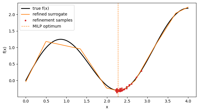
Within a few rounds the MILP optimum moves to the true minimizer, and the true value there matches the true minimum to three decimals. The surrogate’s own prediction at \(x^*\) stays slightly optimistic, at about the noise level of the data. That is expected, because the optimizer always picks the point where the fitted model is lowest.

The plot also shows that the refined surrogate is still coarse away from \(x^*\), around the local maximum near \(x = 1\). That is fine: refinement spends samples only where the answer depends on them.

This is the standard pattern for optimizing over a surrogate: the MILP gives a certified optimum of the model, and new samples make the model accurate at that optimum. The same loop works with real experiments or an expensive simulator in place of f_true.

4. Two inputs

Hinges act on one feature at a time, so a hinge model is a sum of 1-D piecewise-linear functions, one per input (plus categorical terms, shown in section 6). That suits responses that are roughly additive in their inputs. Here is one:

\[f(x_1, x_2) = \tfrac12 (x_1 - 1)^2 (x_1 - 3)^2 + 0.4 x_1 + |x_2 - 2| + 0.3 x_2,\]

which is nonconvex in \(x_1\) (two valleys) and has a kink in \(x_2\).

If your response has strong interactions such as \(x_1 x_2\), an additive hinge model will fit it poorly. You can then add add_interactions() and embed with allow_nonlinear=True, which turns the problem into an MINLP for a solver such as discopt.

def f2_true(x1, x2):
    return 0.5 * (x1 - 1) ** 2 * (x1 - 3) ** 2 + 0.4 * x1 + np.abs(x2 - 2) + 0.3 * x2


X2 = rng.uniform(0, 4, size=(400, 2))
y2 = f2_true(X2[:, 0], X2[:, 1]) + rng.normal(0, 0.02, 400)

library2 = (
    BasisLibrary(n_features=2, feature_names=["x1", "x2"], feature_bounds=[(0, 4), (0, 4)])
    .add_constant()
    .add_linear()
    .add_hinges(X=X2, n_knots=10)
)
model2 = SymbolicRegressor(basis_library=library2, max_terms=14, information_criterion="bic")
model2.fit(X2, y2)
print(f"{len(model2.selected_features_)} terms, R2 = {model2.metrics_['r2']:.4f}")
print("non-MILP terms:", milp_incompatible_terms(model2))

14 terms, R2 = 0.9947
non-MILP terms: []

x_opt2, f_opt2, blk2 = minimize_pyomo(model2)
print("MILP optimum:", x_opt2, f"surrogate = {f_opt2:.4f}, true = {f2_true(**x_opt2):.4f}")

g = np.linspace(0, 4, 201)
A, B = np.meshgrid(g, g)
F_true = f2_true(A, B)
F_sur = np.asarray(model2.predict(np.column_stack([A.ravel(), B.ravel()]))).reshape(A.shape)
i_true = np.argmin(F_true)
print(f"true optimum on grid: x1 = {A.flat[i_true]:.2f}, x2 = {B.flat[i_true]:.2f}, "
      f"f = {F_true.flat[i_true]:.4f}")

fig, axes = plt.subplots(1, 2, figsize=(11, 4.2), sharey=True)
for ax, F, title in zip(axes, (F_true, F_sur), ("true f", "hinge surrogate"), strict=True):
    cs = ax.contourf(A, B, F, levels=30, cmap="viridis")
    ax.plot(x_opt2["x1"], x_opt2["x2"], "r*", ms=16, label="MILP optimum")
    ax.plot(A.flat[i_true], B.flat[i_true], "wx", ms=10, mew=2, label="true optimum")
    ax.set_title(title)
    ax.set_xlabel("x1")
    fig.colorbar(cs, ax=ax)
axes[0].set_ylabel("x2")
axes[0].legend(loc="upper right")
plt.tight_layout()
plt.show()

MILP optimum: {'x1': 0.779284, 'x2': 2.02693} surrogate = 1.0318, true = 1.0668
true optimum on grid: x1 = 0.92, x2 = 2.00, f = 0.9818

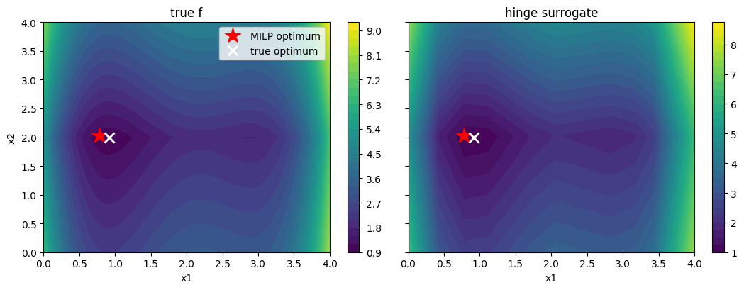
The surrogate reproduces both valleys in \(x_1\) and the kink in \(x_2\), and the MILP lands in the correct (left) valley. The small offset from the true optimum is surrogate error, which section 3’s refinement loop would close.

Fewer binaries with output_sense

Each hinge needs one binary in the exact formulation. When we only ever minimize the output, a hinge with a positive coefficient is convex in the right direction: the solver already pushes it down onto \(\max(0, x - k)\), so it needs no binary. Passing output_sense="min" drops those binaries. We compare the two formulations on a larger model with 20 knots per feature.

library3 = (
    BasisLibrary(n_features=2, feature_names=["x1", "x2"], feature_bounds=[(0, 4), (0, 4)])
    .add_constant()
    .add_linear()
    .add_hinges(X=X2, n_knots=20)
)
model3 = SymbolicRegressor(basis_library=library3, max_terms=25, information_criterion="bic")
model3.fit(X2, y2)
print(f"{len(model3.selected_features_)} terms")

print(f"{'output_sense':>12} {'binaries':>9} {'objective':>10} {'time (s)':>9}")
for sense in (None, "min"):
    t0 = time.perf_counter()
    x_opt3, f_opt3, blk3 = minimize_pyomo(model3, output_sense=sense)
    dt = time.perf_counter() - t0
    print(f"{str(sense):>12} {len(blk3.binaries):9d} {f_opt3:10.5f} {dt:9.3f}")

24 terms
output_sense  binaries  objective  time (s)

        None        23    0.99754     0.017

         min         7    0.99754     0.032

Both formulations give the same optimum, and the relaxed one has fewer binaries. At this size HiGHS solves either in a fraction of a second, but the saving grows with the number of hinges and with embedded models that sit inside bigger problems.

Use output_sense only when it is valid. It is correct only if the output appears solely in a minimized objective (for "min") or solely in a maximized one (for "max"). If the output also appears in a constraint such as cost >= 2, the relaxed hinges can float upward, and the answer is wrong. The default, output_sense=None, is exact in any problem.

5. A design problem with discrete decisions, in Pyomo and discopt

Real problems embed the surrogate among other variables and constraints. We treat model2 as the operating cost of a unit and add the following:

• an operating constraint \(x_1 + x_2 \ge 4\),

• an optional upgrade, a binary \(u\) with fixed cost 0.3, that relaxes the constraint to \(x_1 + x_2 \ge 3\).

The solver has to trade off the upgrade cost against cheaper operation. We pass our own variables through inputs= and output=, and the embedding links them with equality constraints.

m = pyo.ConcreteModel()
m.x1 = pyo.Var(bounds=(0, 4))
m.x2 = pyo.Var(bounds=(0, 4))
m.cost = pyo.Var()
m.u = pyo.Var(within=pyo.Binary)
m.sr = pyo.Block()
model2.to_pyomo(m.sr, inputs={"x1": m.x1, "x2": m.x2}, output=m.cost)

m.spec = pyo.Constraint(expr=m.x1 + m.x2 >= 4 - m.u)
m.obj = pyo.Objective(expr=m.cost + 0.3 * m.u, sense=pyo.minimize)
highs.solve(m)

print(f"Pyomo/HiGHS: x1 = {pyo.value(m.x1):.4f}, x2 = {pyo.value(m.x2):.4f}, "
      f"upgrade = {round(pyo.value(m.u))}, total = {pyo.value(m.obj):.5f}")

Pyomo/HiGHS: x1 = 0.9731, x2 = 2.0269, upgrade = 1, total = 1.36210

The same model in discopt. to_discopt returns a DiscoptEmbedding whose inputs and output are discopt variables, so we can write constraints on them directly. Every variable it creates is named with a prefix (default "jaxsr"), which lets several surrogates live in one model.

dm_model = discopt.Model("design")
emb = model2.to_discopt(dm_model)
u = dm_model.binary("upgrade")
dm_model.subject_to(emb.inputs["x1"] + emb.inputs["x2"] >= 4 - u)
dm_model.minimize(emb.output + 0.3 * u)
result = dm_model.solve()

print(f"discopt: status = {result.status}, total = {result.objective:.5f}")
print(f"agrees with Pyomo: {abs(result.objective - pyo.value(m.obj)) < 1e-5}")

discopt: status = optimal, total = 1.36210

agrees with Pyomo: True

6. Choosing a catalyst: categorical inputs

Categorical inputs become one-hot binaries in the embedding, so a “which option?” decision becomes part of the MILP. Here the yield of a reaction depends on temperature \(T \in [300, 400]\) K and which of three catalysts is used. Each catalyst has its own baseline and temperature slope, and every catalyst loses yield above about 370 K (a hinge). The catalysts also have different costs.

catalysts = ["Pt", "Pd", "Ni"]
base = np.array([0.60, 0.55, 0.30])
slope = np.array([0.10, 0.25, 0.45])          # yield gain per 100 K
cat_cost = {"Pt": 0.20, "Pd": 0.10, "Ni": 0.0}


def yield_true(c, T):
    t = (T - 300) / 100
    return base[c] + slope[c] * t - 1.2 * np.maximum(0, T - 370) / 100


c = rng.integers(0, 3, 300)
T = rng.uniform(300, 400, 300)
Xc = np.column_stack([c, T]).astype(float)
yc = yield_true(c, T) + rng.normal(0, 0.005, 300)

library_c = (
    BasisLibrary(
        n_features=2,
        feature_names=["catalyst", "T"],
        feature_types=["categorical", "continuous"],
        categories={0: catalysts},
        feature_bounds=[(0, 2), (300, 400)],
    )
    .add_constant()
    .add_linear()
    .add_categorical_indicators()
    .add_categorical_interactions()
    .add_hinges(X=Xc, n_knots=9)
)
model_c = SymbolicRegressor(basis_library=library_c, max_terms=8, information_criterion="bic")
model_c.fit(Xc, yc)
print(model_c.expression_)
print("non-MILP terms:", milp_incompatible_terms(model_c))

y = 0.7191 - 1.124*I(catalyst=Ni) - 2.9768e-05*max(0,T-380.064) + 0.002851*I(catalyst=Ni)*T + 0.0006223*max(0,343.177-T) - 0.01021*max(0,T-366.382) - 0.002236*max(0,380.064-T) + 6.0966e-05*I(catalyst=Pd)*T
non-MILP terms: []

We maximize yield minus catalyst cost. jaxsr_onehot[("catalyst", name)] is the binary that is 1 when that catalyst is chosen, so the cost term is just a linear expression in those binaries.

blk = model_c.to_pyomo()
blk.profit = pyo.Objective(
    expr=blk.jaxsr_output - sum(cat_cost[n] * blk.jaxsr_onehot[("catalyst", n)] for n in catalysts),
    sense=pyo.maximize,
)
highs.solve(blk)
chosen = [n for n in catalysts if pyo.value(blk.jaxsr_onehot[("catalyst", n)]) > 0.5][0]
T_opt = pyo.value(blk.jaxsr_inputs["T"])
print(f"MILP: catalyst = {chosen}, T = {T_opt:.1f} K, profit = {pyo.value(blk.profit):.4f}")

# Brute-force check on the surrogate: every catalyst on a fine T grid.
Tg = np.linspace(300, 400, 2001)
for k, name in enumerate(catalysts):
    pred = np.asarray(model_c.predict(np.column_stack([np.full_like(Tg, k), Tg])))
    profit = pred - cat_cost[name]
    print(f"  {name}: best T = {Tg[profit.argmax()]:.1f} K, profit = {profit.max():.4f}")

MILP: catalyst = Pd, T = 366.4 K, profit = 0.6108
  Pt: best T = 366.4 K, profit = 0.4884
  Pd: best T = 366.4 K, profit = 0.6108
  Ni: best T = 366.4 K, profit = 0.6088

The MILP picks the same catalyst and temperature as brute-force enumeration of the surrogate. With three catalysts and one temperature, enumeration is cheap. With several categorical decisions and many continuous inputs it is not, and that is where the MILP formulation pays off.

Summary

The workflow is:

1. Fit with a piecewise-linear library. Use add_constant, add_linear, add_hinges and, if you need them, add_transcendental(["abs"]) and the categorical builders. Place knots where the response bends, or let data quantiles place them.

2. Check that milp_incompatible_terms(model) == [].

3. Embed with model.to_pyomo(block, inputs=..., output=...) or model.to_discopt(dm_model, ...), and add your own objective and constraints.

4. Verify the optimum against the real system and refine there. The MILP certifies the surrogate’s optimum, not the truth’s.

Input bounds come from bounds=, then feature_bounds, then the training data, and the embedding enforces them so the optimizer cannot exploit extrapolation. See the MIP embedding guide for the formulations and every option, including allow_nonlinear=True for MINLP surrogates.