
Time–Temperature Superposition: Learning the Shift Law#
A family of curves indexed by a condition is one of the most common shapes in experimental science. Rheology measures a modulus against frequency at a dozen temperatures; the claim is that shifting each isotherm along the log-frequency axis collapses them all onto a single master curve.
The shift factors are numbers. The law relating them to temperature — Arrhenius, WLF, a polynomial — is traditionally a guess, asserted after the fact.
This notebook uses SuperpositionRegressor to learn that law symbolically, and then
does the thing that matters more: tests whether the collapse actually holds.
Three things to watch for, because each one contradicts an intuition:
The transform is identifiable but the equation is not.
A collapse that looks acceptable by eye can be worthless — the eye has no noise floor.
Expression stability is anti-correlated with validity.
1. Synthetic data with a known answer#
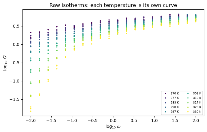
We build a generalized Maxwell storage modulus, measured at 10 temperatures with 3 replicates each and 3% multiplicative noise. The true shift law is Arrhenius with \(E = 55.9\) kJ/mol.
Because we generated it, we know the right answer — which is the only way to tell whether the machinery works.
import warnings

import matplotlib.pyplot as plt
import numpy as np

from jaxsr import SuperpositionRegressor, collapse_rmse

R = 8.314462618          # J/(mol K)
T_REF = 300.0            # reference temperature, K
E_TRUE = 55.9e3          # true activation energy, J/mol

rng = np.random.RandomState(0)
relaxation_times = np.logspace(-2, 2, 6)


def true_log_shift(temperature, energy=E_TRUE):
    '''Arrhenius log10(a_T), anchored at T_REF.'''
    temperature = np.asarray(temperature, dtype=float)
    return energy / (np.log(10) * R) * (1.0 / temperature - 1.0 / T_REF)


def storage_modulus(log_omega, taus=relaxation_times):
    '''log10 G' for a generalized Maxwell model on a log-frequency axis.'''
    w = 10.0**log_omega
    return np.log10(sum((w * t) ** 2 / (1 + (w * t) ** 2) for t in taus))


temperatures = np.linspace(270.0, 330.0, 10)
log_omega_grid = np.linspace(-2.0, 2.0, 20)
NOISE = 0.03

rows = {"temperature": [], "log_omega": [], "log_Gp": []}
for temperature in temperatures:
    shift = float(true_log_shift(temperature))
    for _ in range(3):                                    # replicates -> a real noise floor
        values = storage_modulus(log_omega_grid + shift)
        rows["temperature"].extend([temperature] * log_omega_grid.size)
        rows["log_omega"].extend(log_omega_grid)
        rows["log_Gp"].extend(values + rng.normal(0.0, NOISE, log_omega_grid.size))

data = {k: np.asarray(v) for k, v in rows.items()}
print(f"{data['log_Gp'].size} rows, {len(temperatures)} temperatures, 3 replicates each")
600 rows, 10 temperatures, 3 replicates each
Those replicates are worth the effort. They give a direct estimate of the measurement noise, and every verdict below is a ratio against that noise floor. Without them the floor has to be inferred from curve smoothing, which is weaker.
fig, ax = plt.subplots(figsize=(7, 4.5))
colors = plt.cm.viridis(np.linspace(0, 1, len(temperatures)))
for color, temperature in zip(colors, temperatures):
    mask = data["temperature"] == temperature
    ax.plot(data["log_omega"][mask], data["log_Gp"][mask], ".",
            color=color, ms=4, label=f"{temperature:.0f} K")
ax.set_xlabel(r"$\log_{10}\,\omega$")
ax.set_ylabel(r"$\log_{10}\,G'$")
ax.set_title("Raw isotherms: each temperature is its own curve")
ax.legend(fontsize=7, ncol=2)
fig.tight_layout()
2. Fit#
Note what has to be declared rather than guessed:
domain="frequency"fixes the sign convention (\(z = x + s\)). This names the transform rather than changing it — the collapse is identical either way, so getting it wrong flips the sign of every shift factor and of the activation energy while every plot still looks perfect.condition_scale="kelvin"declares the condition is an absolute temperature. That enables the reciprocal-condition families and rejects a Celsius-looking column.The abscissa is already in log units. The module does not take logs for you.
validation="loco" turns on leave-one-condition-out validation, which is the verdict.
model = SuperpositionRegressor(
    condition="temperature",
    abscissa="log_omega",
    response="log_Gp",
    domain="frequency",
    condition_scale="kelvin",
    reference=T_REF,
    candidate_families=("arrhenius", "wlf", "polynomial"),
    max_terms=2,
    validation="loco",
    max_holdout_conditions=4,
)

with warnings.catch_warnings():
    warnings.simplefilter("ignore")
    model.fit(data)

print(model.summary())
SuperpositionRegressor
==============================================
domain            : frequency (z = x + s(c))
reference         : 300
channels          : ['log_Gp']
conditions        : 10

Transform (the identified quantity)
----------------------------------------------
           270  ->  +1.0406
       276.667  ->  +0.7912
       283.333  ->  +0.5528
           290  ->  +0.3245
       296.667  ->  +0.1059
       303.333  ->  -0.1037
           310  ->  -0.3049
       316.667  ->  -0.4982
       323.333  ->  -0.6840
           330  ->  -0.8627
  effective activation energy : 54.2 kJ/mol

Selected law (not the headline -- see shift_expression_ notes)
----------------------------------------------
  s(q) = -10.798*(q/(1.06991*(1.06991 + q)))

Superposition validity
==============================================
verdict              : supported
noise floor          : 0.03016 (from replicates)
in-sample collapse   : 0.03037
held-out collapse    : 0.03178 (1.05 x noise floor, 4 conditions)
held-out shift error : 0.01625
thresholds           : supported <= 2x, weakly <= 4x noise floor
3. Finding #1 — the transform is identifiable, the equation is not#
Compare what was recovered against the truth.
recovered = model.shift_factors(temperatures)
truth = true_log_shift(temperatures)
error = np.abs(recovered - truth)

print(f"{'T (K)':>8} {'recovered':>11} {'true':>9} {'|error|':>9}")
for temperature, got, want, err in zip(temperatures, recovered, truth, error):
    print(f"{temperature:8.1f} {got:11.4f} {want:9.4f} {err:9.4f}")
print(f"\nmedian |error| = {np.median(error):.4f} decades")
print(f"max    |error| = {np.max(error):.4f} decades   (acceptance criterion: 0.15)")
   T (K)   recovered      true   |error|
   270.0      1.0406    1.0814    0.0409
   276.7      0.7912    0.8208    0.0296
   283.3      0.5528    0.5725    0.0198
   290.0      0.3245    0.3356    0.0111
   296.7      0.1059    0.1094    0.0034
   303.3     -0.1037   -0.1070    0.0032
   310.0     -0.3049   -0.3140    0.0090
   316.7     -0.4982   -0.5123    0.0141
   323.3     -0.6840   -0.7024    0.0184
   330.0     -0.8627   -0.8848    0.0221

median |error| = 0.0162 decades
max    |error| = 0.0409 decades   (acceptance criterion: 0.15)
print("Selected law :", model.shift_expression_)
print(f"E_eff        : {model.effective_activation_energy() / 1000:.1f} kJ/mol")
print(f"true E       : {E_TRUE / 1000:.1f} kJ/mol")
Selected law : -10.798*(q/(1.06991*(1.06991 + q)))
E_eff        : 54.2 kJ/mol
true E       : 55.9 kJ/mol
The data was generated from a pure Arrhenius law, and the Arrhenius basis (\(1/(1+q)^2\)) was in the library. Look at which term was actually selected.
Over a realistic 60 K window, \(1/(1+q)^2\), \(1/(c_2+q)^2\) and low-order polynomials span nearly the same function space — and Arrhenius is the WLF term at \(c_2 = 1\). No information criterion can separate them, so the selected structure is close to arbitrary among near-equivalent forms, while the transform it encodes is pinned down.
In the study behind this module only 62% of 90 fits selected the true Arrhenius basis; the other 38% picked one of nine distinct structural forms — all producing the same transform to ~0.01 decades.
So report shift_factors() and effective_activation_energy(). Do not report
shift_expression_. The effective activation energy is the useful summary precisely
because it is comparable across structurally different fits.
4. The collapse#
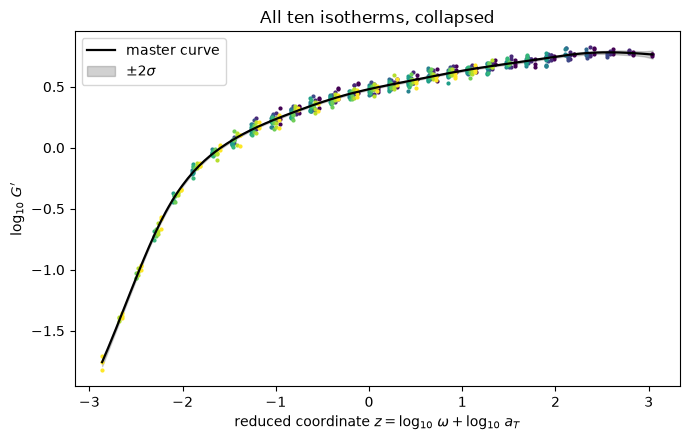
Apply the transform and rebuild the master curve.
reduced = model.transform()
master = model.master_curve_["log_Gp"]

fig, ax = plt.subplots(figsize=(7, 4.5))
for color, temperature in zip(colors, temperatures):
    mask = reduced["temperature"] == temperature
    ax.plot(reduced["z"][mask], reduced["w"][mask], ".", color=color, ms=4)
ax.plot(master.z, master.y, "k-", lw=1.6, label="master curve")
ax.fill_between(master.z, master.y - 2 * master.std, master.y + 2 * master.std,
                color="k", alpha=0.18, label=r"$\pm 2\sigma$")
ax.set_xlabel(r"reduced coordinate $z = \log_{10}\,\omega + \log_{10}\,a_T$")
ax.set_ylabel(r"$\log_{10}\,G'$")
ax.set_title("All ten isotherms, collapsed")
ax.legend()
fig.tight_layout()
print(f"collapse RMSE : {collapse_rmse(reduced['z'], reduced['w']):.4f}")
print(f"noise floor   : {model.noise_floor_:.4f}  (from {model.noise_floor_source_})")
collapse RMSE : 0.0304
noise floor   : 0.0302  (from replicates)
5. Finding #2 — a beautiful collapse proves nothing#
Now the important part. We build a thermorheologically complex material: two relaxation groups with different activation energies, so no single scalar shift factor can collapse the family. There is no valid transform, and the honest answer is “this does not superpose.”
taus_fast, taus_slow = np.logspace(-1.5, -0.5, 3), np.logspace(0.5, 1.5, 3)
rng_bad = np.random.RandomState(0)
temps_bad = np.linspace(T_REF - 50, T_REF + 50, 10)

rows_bad = {"temperature": [], "log_omega": [], "log_Gp": []}
for temperature in temps_bad:
    a_fast = float(true_log_shift(temperature, 10e3))     # 10 kJ/mol
    a_slow = float(true_log_shift(temperature, 180e3))    # 180 kJ/mol -- different!
    for _ in range(2):
        w_fast = 10.0 ** (log_omega_grid + a_fast)
        w_slow = 10.0 ** (log_omega_grid + a_slow)
        modulus = sum((w_fast * t) ** 2 / (1 + (w_fast * t) ** 2) for t in taus_fast)
        modulus += sum((w_slow * t) ** 2 / (1 + (w_slow * t) ** 2) for t in taus_slow)
        rows_bad["temperature"].extend([temperature] * log_omega_grid.size)
        rows_bad["log_omega"].extend(log_omega_grid)
        rows_bad["log_Gp"].extend(np.log10(modulus) + rng_bad.normal(0.0, NOISE, log_omega_grid.size))

data_bad = {k: np.asarray(v) for k, v in rows_bad.items()}

model_bad = SuperpositionRegressor(
    condition="temperature", abscissa="log_omega", response="log_Gp",
    domain="frequency", condition_scale="kelvin", reference=T_REF,
    max_terms=2, validation="loco", max_holdout_conditions=3,
)
with warnings.catch_warnings():
    warnings.simplefilter("ignore")
    model_bad.fit(data_bad)

print("It still returns a confident shift law:")
print(" ", model_bad.shift_expression_)
It still returns a confident shift law:
  1321.83*(q**3/3) + -11.4007*(q/(0.620922*(0.620922 + q)))
reduced_bad = model_bad.transform()
master_bad = model_bad.master_curve_["log_Gp"]

fig, axes = plt.subplots(1, 2, figsize=(11, 4.2), sharey=True)
for ax, red, mast, title in (
    (axes[0], reduced, master, "Genuine superposition"),
    (axes[1], reduced_bad, master_bad, "No valid transform exists"),
):
    ax.plot(red["z"], red["w"], ".", ms=3, alpha=0.5, color="tab:blue")
    ax.plot(mast.z, mast.y, "k-", lw=1.5)
    ax.set_xlabel("reduced coordinate $z$")
    ax.set_title(title)
axes[0].set_ylabel(r"$\log_{10}\,G'$")
fig.suptitle("Right: still reads as a master curve. Its scatter is 6x the noise floor.", y=1.02)
fig.tight_layout()
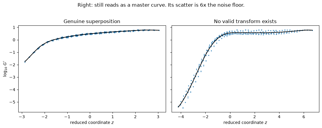
The right panel still reads as a master curve with some experimental scatter. On a plot spanning seven decades of \(G'\), a spread of 0.18 is easy to wave through — and that is the trap: the eye cannot supply the noise floor. Those replicates put the measurement noise at 0.030, so 0.18 is six times larger than anything the data can excuse.
That is the first reason to distrust a visual collapse. The second is that the in-sample number is computed against a master curve fitted to the very rows being scored, so it flatters the model. A temperature withheld from the entire pipeline does not: it takes no part in the smoothing or in the discovery, and is shifted by prediction alone.
for label, m in (("genuine ", model), ("complex ", model_bad)):
    r = m.validity_report_
    print(f"{label}: verdict={r.verdict:17s} "
          f"in-sample={r.in_sample_collapse:.4f}  "
          f"held-out={r.holdout_collapse_median:.4f}  "
          f"({r.holdout_ratio_median:.2f}x noise floor)")
genuine : verdict=supported         in-sample=0.0304  held-out=0.0318  (1.05x noise floor)
complex : verdict=not_supported     in-sample=0.1799  held-out=0.2305  (7.91x noise floor)
Both collapses degrade, but the held-out number is the more sensitive test (7.9x against 6.2x in-sample) and the more trustworthy one, for the reason above.
validity_report_ grades on multiples of the measured noise floor: <= 2x supported,
<= 4x weakly supported, beyond that not supported. Notice how much work the noise floor
is doing — without replicates to calibrate it, 0.18 is just a number.
print(model_bad.validity_report_.summary())
print()
print("Per-withheld-condition detail (complex case):")
for entry in model_bad.validity_report_.holdout:
    print(f"  T={entry['condition']:6.1f} K  collapse={entry['collapse_rmse']:.4f} "
          f"({entry['ratio']:5.2f}x)  predicted shift={entry['shift_predicted']:+.3f} "
          f"best-aligning={entry['shift_aligned']:+.3f}")
Superposition validity
==============================================
verdict              : not_supported
noise floor          : 0.02913 (from replicates)
in-sample collapse   : 0.1799
held-out collapse    : 0.2305 (7.91 x noise floor, 3 conditions)
held-out shift error : 0.8025
thresholds           : supported <= 2x, weakly <= 4x noise floor

Per-withheld-condition detail (complex case):
  T= 250.0 K  collapse=0.2305 ( 7.91x)  predicted shift=+9.224 best-aligning=+7.674
  T= 294.4 K  collapse=0.1855 ( 6.37x)  predicted shift=+0.520 best-aligning=+0.790
  T= 350.0 K  collapse=1.1942 (40.99x)  predicted shift=-1.366 best-aligning=-2.169
That last column is a diagnosis, not decoration. Each withheld curve also reports the shift that would have aligned it best:
|
|
Meaning |
|---|---|---|
large |
large |
the law extrapolated wrongly — more conditions, or a different family |
small |
large |
the curve does not collapse under any shift — superposition fails |
Here the predicted and best-aligning shifts are close while the collapse is still bad, which is the second row: no scalar shift factor exists.
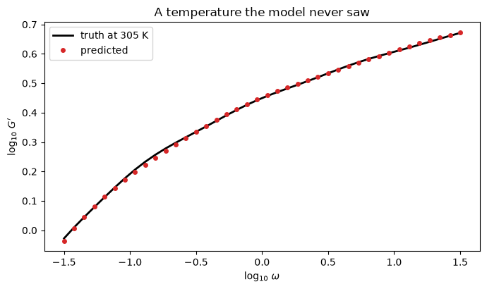
7. The payoff: predicting an unmeasured temperature#
Because the shift law is symbolic, it extrapolates. Classic superposition tooling returns a table of per-curve shift factors and simply cannot answer this.
unmeasured = 305.0                        # never in the training data
assert unmeasured not in temperatures

x_new = np.linspace(-1.5, 1.5, 40)
predicted = model.predict(np.full(x_new.size, unmeasured), x_new)
expected = storage_modulus(x_new + true_log_shift(unmeasured))

fig, ax = plt.subplots(figsize=(7, 4.2))
ax.plot(x_new, expected, "k-", lw=2, label=f"truth at {unmeasured:.0f} K")
ax.plot(x_new, predicted, "o", ms=4, color="tab:red", label="predicted")
ax.set_xlabel(r"$\log_{10}\,\omega$")
ax.set_ylabel(r"$\log_{10}\,G'$")
ax.set_title("A temperature the model never saw")
ax.legend()
fig.tight_layout()

print(f"shift at {unmeasured:.0f} K : predicted {model.shift_factors([unmeasured])[0]:+.4f}, "
      f"true {true_log_shift(unmeasured):+.4f}")
print(f"prediction RMSE   : {np.sqrt(np.mean((predicted - expected) ** 2)):.4f}")
shift at 305 K : predicted -0.1548, true -0.1596
prediction RMSE   : 0.0044
Summary#
Question |
Answer |
|---|---|
What is the shift at temperature \(T\)? |
|
What is the physics? |
|
What is the equation? |
|
Does the collapse hold? |
|
How reproducible is the search? |
|
The one habit worth carrying away: a collapse you can see is not evidence. Only a condition withheld from the whole pipeline is.
See also#
Structured basis blocks — the
Θ(q) ⊙ y_xmachinery underneathMultivariate derivative estimation — the derivative stage
Resampling and stability — why the ensemble re-runs the smoother