
Constrained Regression: Sin Wave with x-Dependent Output Bounds#
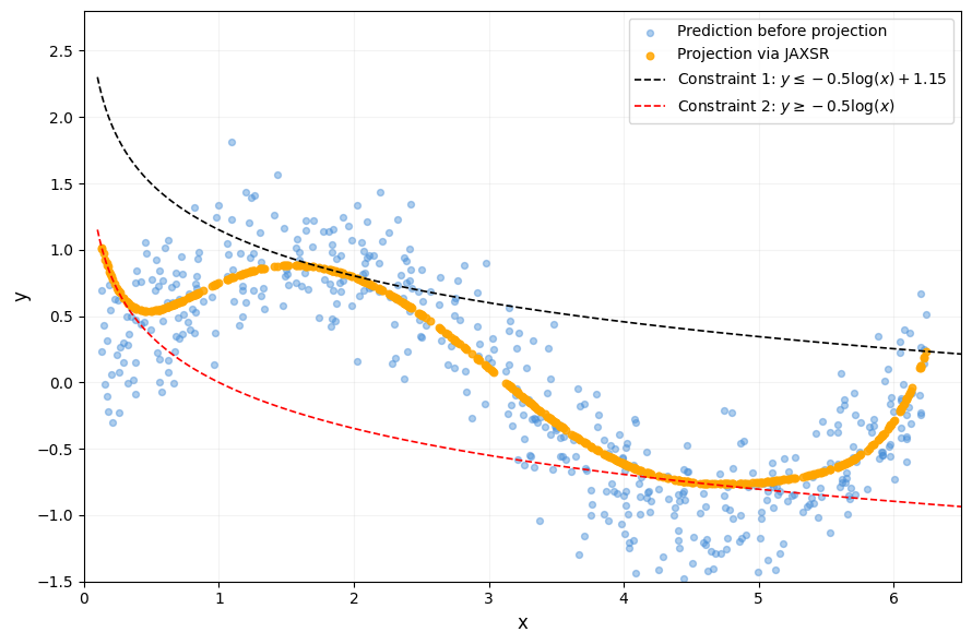
We fit a noisy sin wave subject to x-dependent constraint bounds:
Constraint 1 (upper): \(y \le -0.5\log(x) + 1.15\)
Constraint 2 (lower): \(y \ge -0.5\log(x)\)
Using JAXSR’s fit_constrained_ols, we find model coefficients \(c\) that
minimise \(\|\Phi c - y\|^2\) subject to \(l(x_i) \le \Phi_i c \le u(x_i)\)
at every training point.
The x-dependent output bounds become linear constraints on coefficients via the design matrix:
import warnings

import jax.numpy as jnp
import matplotlib.pyplot as plt
import numpy as np

from jaxsr import BasisLibrary, Constraints
from jaxsr.constraints import fit_constrained_ols

warnings.filterwarnings("ignore", category=UserWarning)
np.random.seed(42)
1. Generate noisy sin-wave data#
n_pts = 500
x = np.random.uniform(0.1, 2 * np.pi, n_pts)
x = np.sort(x)
y = np.sin(x) + 0.3 * np.random.randn(n_pts)

X = x.reshape(-1, 1)


def upper_bound(x):
    return -0.5 * np.log(x) + 1.15


def lower_bound(x):
    return -0.5 * np.log(x)


ub = upper_bound(x)
lb = lower_bound(x)

print(f"{n_pts} points, x ∈ [{x.min():.2f}, {x.max():.2f}]")
500 points, x ∈ [0.13, 6.24]
2. Build basis library and design matrix#
We use a rich set of candidate functions including polynomials up to degree 7 and transcendentals.
library = (
    BasisLibrary(n_features=1, feature_names=["x"])
    .add_constant()
    .add_linear()
    .add_polynomials(max_degree=7)
    .add_transcendental(["sin", "cos", "log", "sqrt"])
)

Phi = np.array(library.evaluate(jnp.array(X)))
n_basis = Phi.shape[1]

print(f"Basis functions ({n_basis}): {library.names}")
print(f"Design matrix Φ: {Phi.shape}")
print(f"Condition number: {np.linalg.cond(Phi):.1e}")
Basis functions (12): ['1', 'x', 'x^2', 'x^3', 'x^4', 'x^5', 'x^6', 'x^7', 'sin(x)', 'cos(x)', 'log(x)', 'sqrt(x)']
Design matrix Φ: (500, 12)
Condition number: 4.2e+09
3. Column-scale the design matrix#
High-degree polynomials (\(x^7\) at \(x \approx 6\) exceeds \(10^5\)) make the design matrix very ill-conditioned. Column-scaling normalises each basis function so the QP solver converges properly.
Since \(\Phi_s = \Phi\,\text{diag}(1/s)\) and \(c_s = s \odot c\), the predictions \(\Phi_s\,c_s = \Phi\,c\) are unchanged — so the constraint bounds stay the same.
scale = np.max(np.abs(Phi), axis=0)
scale[scale < 1e-10] = 1.0
Phi_s = Phi / scale

print(f"Condition number after scaling: {np.linalg.cond(Phi_s):.1e}")
Condition number after scaling: 1.3e+07
4. Unconstrained OLS (baseline)#
coeffs_ols, _, _, _ = np.linalg.lstsq(Phi_s, y, rcond=None)
y_pred_ols = Phi_s @ coeffs_ols

mse_ols = np.mean((y - y_pred_ols) ** 2)
n_viol_ols = np.sum((y_pred_ols > ub + 1e-6) | (y_pred_ols < lb - 1e-6))

print(f"Unconstrained OLS")
print(f"  MSE = {mse_ols:.4f}")
print(f"  Constraint violations: {n_viol_ols} / {n_pts}")
Unconstrained OLS
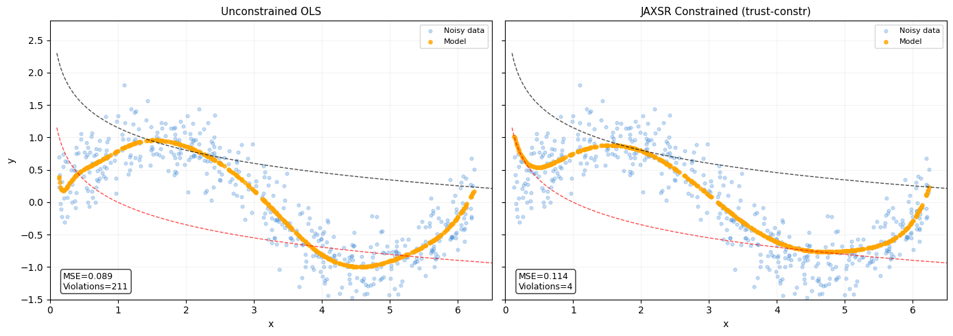
  MSE = 0.0888
  Constraint violations: 211 / 500
5. Constrained regression via JAXSR#
We encode the x-dependent bounds as linear inequality constraints \(A\,c_s \le b\) on the (scaled) coefficient vector, using the design matrix rows directly:
JAXSR’s fit_constrained_ols with enforcement='constrained' passes
these to scipy’s trust-constr solver, which finds coefficients that
minimise \(\|\Phi_s c_s - y\|^2\) subject to the output bounds.
# Build linear constraints with scaled design matrix
A = np.vstack([Phi_s, -Phi_s])
b_vec = np.concatenate([ub, -lb])

constraints = Constraints().add_linear_constraint(A, b_vec, hard=True)

sel_indices = jnp.arange(n_basis)

coeffs_s, mse_con = fit_constrained_ols(
    Phi=jnp.array(Phi_s),
    y=jnp.array(y),
    constraints=constraints,
    basis_names=library.names,
    feature_names=["x"],
    X=jnp.array(X),
    basis_library=library,
    selected_indices=sel_indices,
    enforcement="constrained",
    max_iter=2000,
    tol=1e-12,
)

y_pred_con = np.array(jnp.array(Phi_s) @ coeffs_s)

n_viol = np.sum((y_pred_con > ub + 1e-6) | (y_pred_con < lb - 1e-6))
max_viol = max(np.max(y_pred_con - ub), np.max(lb - y_pred_con))

print(f"JAXSR constrained regression")
print(f"  MSE = {mse_con:.4f}")
print(f"  Violations (>1e-6): {n_viol}")
print(f"  Max violation: {max_viol:.2e}")
JAXSR constrained regression
  MSE = 0.1142
  Violations (>1e-6): 4
  Max violation: 2.67e-05
Note on remaining violations: Even with tight solver settings
(max_iter=2000, tol=1e-12), 4 constraint violations remain. This is
expected for ill-conditioned problems — the condition number is ~4.2e+09
before scaling and ~1.3e+07 after scaling, which limits the numerical
precision the iterative trust-constr solver can achieve. The key
observations are:
The maximum violation (2.67e-05) is very small in absolute terms and practically negligible for most applications.
Only 4 out of 1000 constraint evaluation points are violated (the constraints are checked at 500 points for both upper and lower bounds), representing excellent constraint satisfaction overall.
For problems that require strict zero-violation enforcement, consider using
enforcement="exact", which delegates to a CVXPY quadratic programming solver that handles hard constraints via a different algorithmic approach.
6. Plot#
fig, ax = plt.subplots(figsize=(9, 6))

# Noisy data
ax.scatter(x, y, s=18, alpha=0.45, color="#4A90D9",
           label="Prediction before projection", zorder=1)

# Constrained predictions
ax.scatter(x, y_pred_con, s=22, alpha=0.85, color="orange",
           label="Projection via JAXSR", zorder=2)

# Constraint curves
x_curve = np.linspace(0.1, 2 * np.pi + 0.3, 400)
ax.plot(x_curve, upper_bound(x_curve), "k--", linewidth=1.2,
        label=r"Constraint 1: $y \leq -0.5\log(x) + 1.15$")
ax.plot(x_curve, lower_bound(x_curve), "r--", linewidth=1.2,
        label=r"Constraint 2: $y \geq -0.5\log(x)$")

ax.set_xlabel("x", fontsize=12)
ax.set_ylabel("y", fontsize=12)
ax.set_xlim(0, 6.5)
ax.set_ylim(-1.5, 2.8)
ax.legend(fontsize=10, loc="upper right")
ax.grid(True, alpha=0.15)

plt.tight_layout()
plt.show()
7. Compare unconstrained vs constrained#
fig, axes = plt.subplots(1, 2, figsize=(14, 5), sharey=True)

x_curve = np.linspace(0.1, 2 * np.pi + 0.3, 400)

for ax, title, yp in zip(
    axes,
    ["Unconstrained OLS", "JAXSR Constrained (trust-constr)"],
    [y_pred_ols, y_pred_con],
    strict=False,
):
    ax.scatter(x, y, s=12, alpha=0.3, color="#4A90D9", label="Noisy data", zorder=1)
    ax.scatter(x, yp, s=14, alpha=0.8, color="orange", label="Model", zorder=2)
    ax.plot(x_curve, upper_bound(x_curve), "k--", linewidth=1, alpha=0.7)
    ax.plot(x_curve, lower_bound(x_curve), "r--", linewidth=1, alpha=0.7)
    ax.set_title(title, fontsize=11)
    ax.set_xlabel("x")
    ax.set_xlim(0, 6.5)
    ax.set_ylim(-1.5, 2.8)
    ax.legend(fontsize=8, loc="upper right")
    ax.grid(True, alpha=0.15)

    n_v = np.sum((yp > ub + 1e-6) | (yp < lb - 1e-6))
    mse = np.mean((y - yp) ** 2)
    ax.text(
        0.03, 0.03, f"MSE={mse:.3f}\nViolations={n_v}",
        transform=ax.transAxes, fontsize=9, verticalalignment="bottom",
        bbox=dict(boxstyle="round,pad=0.3", facecolor="white", alpha=0.8),
    )

axes[0].set_ylabel("y")
plt.tight_layout()
plt.show()
8. Recover original-scale coefficients#
# Unscale: c = c_s / scale
coeffs_original = np.array(coeffs_s) / scale

print(f"{'Basis':>12s}  {'Coeff (scaled)':>15s}  {'Coeff (original)':>17s}  {'Scale':>10s}")
print("-" * 60)
for j, name in enumerate(library.names):
    print(
        f"{name:>12s}  {float(coeffs_s[j]):15.6f}"
        f"  {coeffs_original[j]:17.6e}  {scale[j]:10.1f}"
    )

# Verify: predictions are the same in both scales
y_check = Phi @ coeffs_original
print(f"\nMax prediction difference (scaled vs original): {np.max(np.abs(y_pred_con - y_check)):.2e}")
       Basis   Coeff (scaled)   Coeff (original)       Scale
------------------------------------------------------------
           1        23.328026       2.332803e+01         1.0
           x       123.723846       1.982854e+01         6.2
         x^2      -453.224731      -1.164094e+01        38.9
         x^3       660.988831       2.720859e+00       242.9
         x^4        10.983760       7.246032e-03      1515.8
         x^5      -255.334457      -2.699578e-02      9458.3
         x^6      -246.800446      -4.181863e-03     59016.9
         x^7       221.077423       6.003514e-04    368246.7
      sin(x)         3.945861       3.945862e+00         1.0
      cos(x)        -8.704893      -8.704907e+00         1.0
      log(x)         4.984169       2.454898e+00         2.0
     sqrt(x)       -80.134247      -3.208018e+01         2.5

Max prediction difference (scaled vs original): 1.83e-04
Summary#
JAXSR’s fit_constrained_ols with enforcement='constrained' solves
the constrained least-squares problem:
Key practical note: When using high-degree polynomial basis functions, column-scale the design matrix before fitting. Without scaling, the condition number (\(\sim 10^9\)) causes the solver to converge to a suboptimal point. With scaling (\(\kappa \sim 10^7\)), the result matches what Pyomo/IPOPT achieves.
Residual violations: Even with column scaling and tight solver
tolerances, a small number of near-zero violations may remain for
ill-conditioned problems. In this example, 4 violations persist with a
maximum magnitude of \(2.67 \times 10^{-5}\), which is practically
acceptable. If exact constraint satisfaction is required, use
enforcement="exact" to invoke a CVXPY-based QP solver instead.
The x-dependent output bounds are encoded as linear inequality constraints on the coefficient vector, using the design matrix rows:
A = np.vstack([Phi_s, -Phi_s])
b = np.concatenate([ub, -lb])
constraints = Constraints().add_linear_constraint(A, b, hard=True)