
Symbolic Classification#
JAXSR can discover interpretable classification models — logistic expressions
that map features to class probabilities. Just as SymbolicRegressor selects
sparse basis functions for regression, SymbolicClassifier selects sparse
basis functions for the linear predictor of a logistic model and fits
coefficients via Iteratively Reweighted Least Squares (IRLS).
Key ideas:
Binary classification: \(P(y=1 \mid x) = \sigma(\Phi(x) \cdot w)\) where \(\sigma\) is the sigmoid function
Multiclass: one-vs-rest (OVR), giving each class its own interpretable expression
Same selection strategies as regression (greedy forward, backward, exhaustive, lasso path)
Information criteria (AIC/BIC/AICc) based on Bernoulli log-likelihood
Full uncertainty quantification: Wald intervals, bootstrap, conformal prediction sets, calibration
import jax.numpy as jnp
import matplotlib.pyplot as plt
import numpy as np
from scipy import stats as sp_stats

from jaxsr import (
    BasisLibrary,
    SymbolicClassifier,
    compute_accuracy,
    compute_auc_roc,
    compute_confusion_matrix,
    compute_f1_score,
    compute_log_loss,
    compute_matthews_corrcoef,
    compute_precision,
    compute_recall,
    fit_symbolic_classification,
)
from jaxsr.uncertainty import (
    bootstrap_classification_coefficients,
    calibration_curve,
)
Binary classification#
We start with a binary classification task where the decision boundary is a quadratic function of two features. The true boundary is:
where \(\sigma(z) = 1 / (1 + e^{-z})\) is the sigmoid function.
# Generate binary classification data with a quadratic boundary
np.random.seed(42)
n_samples = 300
X = np.random.randn(n_samples, 2)

# True logit: 2*x0 - 1.5*x1^2 + 1
logits = 2.0 * X[:, 0] - 1.5 * X[:, 1] ** 2 + 1.0
probs = 1.0 / (1.0 + np.exp(-logits))
y = (np.random.rand(n_samples) < probs).astype(float)

X_jax = jnp.array(X)
y_jax = jnp.array(y)

print(f"True logit: 2*x0 - 1.5*x1^2 + 1")
print(f"Data: {n_samples} samples, 2 features")
print(f"Class balance: {int(y.sum())} positive, {int(n_samples - y.sum())} negative")
True logit: 2*x0 - 1.5*x1^2 + 1
Data: 300 samples, 2 features
Class balance: 145 positive, 155 negative
# Build basis library
library = (
    BasisLibrary(n_features=2, feature_names=["x0", "x1"])
    .add_constant()
    .add_linear()
    .add_polynomials(max_degree=3)
    .add_interactions(max_order=2)
)

print(f"Basis library: {len(library)} candidate functions")
print(f"Candidates: {library.names}")

# Fit classifier
clf = SymbolicClassifier(
    basis_library=library,
    max_terms=5,
    strategy="greedy_forward",
    information_criterion="bic",
)
clf.fit(X_jax, y_jax)

print(f"\nDiscovered linear predictor:")
print(f"  logit = {clf.expression_}")
print(f"\nTraining accuracy: {clf.score(X_jax, y_jax):.4f}")
Basis library: 8 candidate functions
Candidates: ['1', 'x0', 'x1', 'x0^2', 'x0^3', 'x1^2', 'x1^3', 'x0*x1']
Discovered linear predictor:
  logit = y = 1.823*x0 - 1.711*x1^2 + 1.235

Training accuracy: 0.7800
Model diagnostics#
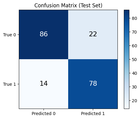
The metrics_ property computes a suite of classification metrics on the
training data. Individual metric functions are also available for use on
held-out data.
# Comprehensive training metrics
metrics = clf.metrics_
print("Training Metrics:")
for name, value in metrics.items():
    print(f"  {name:20s}: {value:.4f}")
Training Metrics:
  accuracy            : 0.7800
  precision           : 0.7762
  recall              : 0.7655
  f1                  : 0.7708
  mcc                 : 0.5594
  log_loss            : 0.4321
  aic                 : 265.2849
  bic                 : 276.3962
  aicc                : 265.3660
  auc_roc             : 0.8763
# Evaluate on held-out test data
np.random.seed(123)
X_test = np.random.randn(200, 2)
logits_test = 2.0 * X_test[:, 0] - 1.5 * X_test[:, 1] ** 2 + 1.0
probs_test = 1.0 / (1.0 + np.exp(-logits_test))
y_test = (np.random.rand(200) < probs_test).astype(float)

X_test_jax = jnp.array(X_test)
y_test_jax = jnp.array(y_test)

y_pred = clf.predict(X_test_jax)
y_proba = clf.predict_proba(X_test_jax)[:, 1]

print("Test Set Metrics:")
print(f"  Accuracy:  {compute_accuracy(y_test_jax, y_pred):.4f}")
print(f"  Precision: {compute_precision(y_test_jax, y_pred):.4f}")
print(f"  Recall:    {compute_recall(y_test_jax, y_pred):.4f}")
print(f"  F1 Score:  {compute_f1_score(y_test_jax, y_pred):.4f}")
print(f"  AUC-ROC:   {compute_auc_roc(y_test_jax, y_proba):.4f}")
print(f"  Log Loss:  {compute_log_loss(y_test_jax, y_proba):.4f}")
print(f"  MCC:       {compute_matthews_corrcoef(y_test_jax, y_pred):.4f}")
Test Set Metrics:
  Accuracy:  0.8200
  Precision: 0.7800
  Recall:    0.8478
  F1 Score:  0.8125
  AUC-ROC:   0.9064
  Log Loss:  0.3888
  MCC:       0.6421
# Confusion matrix
cm = compute_confusion_matrix(y_test_jax, y_pred)

fig, ax = plt.subplots(figsize=(5, 4))
im = ax.imshow(cm, cmap="Blues")
ax.set_xticks([0, 1])
ax.set_yticks([0, 1])
ax.set_xticklabels(["Predicted 0", "Predicted 1"])
ax.set_yticklabels(["True 0", "True 1"])
ax.set_title("Confusion Matrix (Test Set)")

for i in range(2):
    for j in range(2):
        color = "white" if cm[i, j] > cm.max() / 2 else "black"
        ax.text(j, i, str(cm[i, j]), ha="center", va="center", color=color, fontsize=16)

fig.colorbar(im, ax=ax)
plt.tight_layout()
plt.show()
Decision boundary#
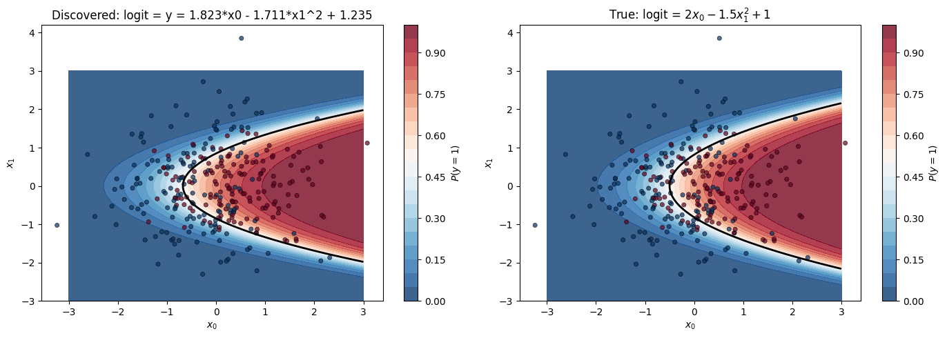
Visualizing the decision boundary in 2D helps us see how the discovered expression partitions the feature space.
# Plot decision boundary
xx, yy = np.meshgrid(
    np.linspace(-3, 3, 200),
    np.linspace(-3, 3, 200),
)
grid = jnp.array(np.column_stack([xx.ravel(), yy.ravel()]))
proba_grid = np.array(clf.predict_proba(grid)[:, 1]).reshape(xx.shape)

fig, axes = plt.subplots(1, 2, figsize=(14, 5))

# Left: discovered boundary
ax = axes[0]
cs = ax.contourf(xx, yy, proba_grid, levels=20, cmap="RdBu_r", alpha=0.8)
ax.contour(xx, yy, proba_grid, levels=[0.5], colors="k", linewidths=2)
scatter = ax.scatter(
    X[:, 0], X[:, 1], c=y, cmap="RdBu_r", edgecolors="k", linewidth=0.5, s=20, alpha=0.7
)
ax.set_xlabel("$x_0$")
ax.set_ylabel("$x_1$")
ax.set_title(f"Discovered: logit = {clf.expression_}")
fig.colorbar(cs, ax=ax, label="$P(y=1)$")

# Right: true boundary for comparison
ax = axes[1]
true_logits = 2.0 * xx - 1.5 * yy**2 + 1.0
true_proba = 1.0 / (1.0 + np.exp(-true_logits))
cs = ax.contourf(xx, yy, true_proba, levels=20, cmap="RdBu_r", alpha=0.8)
ax.contour(xx, yy, true_proba, levels=[0.5], colors="k", linewidths=2)
ax.scatter(
    X[:, 0], X[:, 1], c=y, cmap="RdBu_r", edgecolors="k", linewidth=0.5, s=20, alpha=0.7
)
ax.set_xlabel("$x_0$")
ax.set_ylabel("$x_1$")
ax.set_title("True: logit = $2x_0 - 1.5x_1^2 + 1$")
fig.colorbar(cs, ax=ax, label="$P(y=1)$")

plt.tight_layout()
plt.show()
Selection strategies#
SymbolicClassifier supports the same model-selection strategies as
SymbolicRegressor. Each trades off computation against optimality.
strategies = ["greedy_forward", "greedy_backward", "exhaustive", "lasso_path"]

print(f"{'Strategy':20s} {'Expression':45s} {'Accuracy':>8s}  {'BIC':>8s}")
print("-" * 90)

for strat in strategies:
    m = SymbolicClassifier(
        basis_library=library,
        max_terms=5,
        strategy=strat,
        information_criterion="bic",
    )
    m.fit(X_jax, y_jax)
    expr = m.expression_
    acc = m.score(X_jax, y_jax)
    bic = m.metrics_["bic"]
    print(f"{strat:20s} {expr:45s} {acc:8.4f}  {bic:8.2f}")
Strategy             Expression                                    Accuracy       BIC
------------------------------------------------------------------------------------------
greedy_forward       y = 1.823*x0 - 1.711*x1^2 + 1.235               0.7800    276.40
greedy_backward y = 1.235 + 1.823*x0 - 1.711*x1^2 0.7800 276.40
exhaustive y = 1.235 + 1.823*x0 - 1.711*x1^2 0.7800 276.40
lasso_path y = 1.234 + 1.843*x0 - 0.01065*x0^3 - 1.707*x1^2 0.7800 282.09
Pareto front: complexity vs fit#
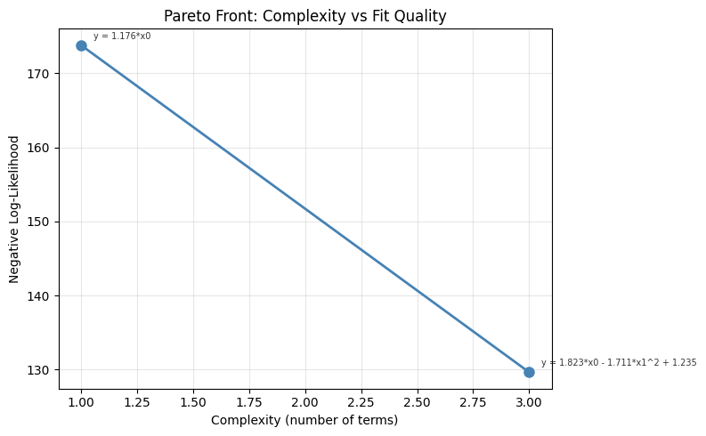
The Pareto front shows the trade-off between model complexity and negative log-likelihood. Simpler models are more interpretable; more complex models fit better.
print("Pareto Front (Complexity vs NLL):")
print(f"{'Complexity':>10s}  {'NLL':>10s}  {'BIC':>10s}  Expression")
print("-" * 80)
for result in clf.pareto_front_:
    print(
        f"{result.complexity:10d}  {result.neg_log_likelihood:10.4f}  "
        f"{result.bic:10.2f}  {result.expression()}"
    )

# Plot the Pareto front
complexities = [r.complexity for r in clf.pareto_front_]
nlls = [r.neg_log_likelihood for r in clf.pareto_front_]

fig, ax = plt.subplots(figsize=(8, 5))
ax.plot(complexities, nlls, "o-", color="steelblue", markersize=8, linewidth=2)
for i, r in enumerate(clf.pareto_front_):
    ax.annotate(
        r.expression(),
        (complexities[i], nlls[i]),
        textcoords="offset points",
        xytext=(10, 5),
        fontsize=7,
        alpha=0.8,
    )
ax.set_xlabel("Complexity (number of terms)")
ax.set_ylabel("Negative Log-Likelihood")
ax.set_title("Pareto Front: Complexity vs Fit Quality")
ax.grid(True, alpha=0.3)
plt.tight_layout()
plt.show()
Pareto Front (Complexity vs NLL):
Complexity         NLL         BIC  Expression
--------------------------------------------------------------------------------
         1    173.7852      353.27  y = 1.176*x0
         3    129.6424      276.40  y = 1.823*x0 - 1.711*x1^2 + 1.235
Coefficient confidence intervals#
For binary classifiers, coefficient_intervals() returns Wald confidence
intervals based on the Fisher information matrix
\(I(w) = \Phi^T \, \text{diag}(\mu(1-\mu)) \, \Phi\), where \(\mu = \sigma(\Phi w)\).
Standard errors come from \(\sqrt{\text{diag}(I^{-1})}\) with Normal quantiles
(MLE asymptotics).
intervals = clf.coefficient_intervals(alpha=0.05)

print("95% Wald Confidence Intervals:")
print(f"  {'Term':>15s} {'Estimate':>10s} {'Std Err':>9s} {'z':>8s} {'p-value':>10s}   95% CI")
print("  " + "-" * 75)
for name, (est, lo, hi, se) in intervals.items():
    z_val = est / se if abs(se) > 1e-15 else float("inf")
    p_val = float(2 * (1 - sp_stats.norm.cdf(abs(z_val))))
    sig = "***" if p_val < 0.001 else ("**" if p_val < 0.01 else ("*" if p_val < 0.05 else ""))
    print(
        f"  {name:>15s} {est:10.4f} {se:9.4f} {z_val:8.2f} {p_val:10.2e}"
        f"   [{lo:.4f}, {hi:.4f}] {sig}"
    )
print("  --- *** p<0.001, ** p<0.01, * p<0.05")
print()
print("Note: Uses Normal quantiles (MLE asymptotics), not t-distribution.")
95% Wald Confidence Intervals:
             Term   Estimate   Std Err        z    p-value   95% CI
  ---------------------------------------------------------------------------
               x0     1.8235    0.2362     7.72   1.15e-14   [1.3606, 2.2863] ***
             x1^2    -1.7111    0.2574    -6.65   3.00e-11   [-2.2157, -1.2065] ***
                1     1.2348    0.2285     5.40   6.53e-08   [0.7869, 1.6826] ***
  --- *** p<0.001, ** p<0.01, * p<0.05

Note: Uses Normal quantiles (MLE asymptotics), not t-distribution.
Bootstrap coefficient uncertainty#
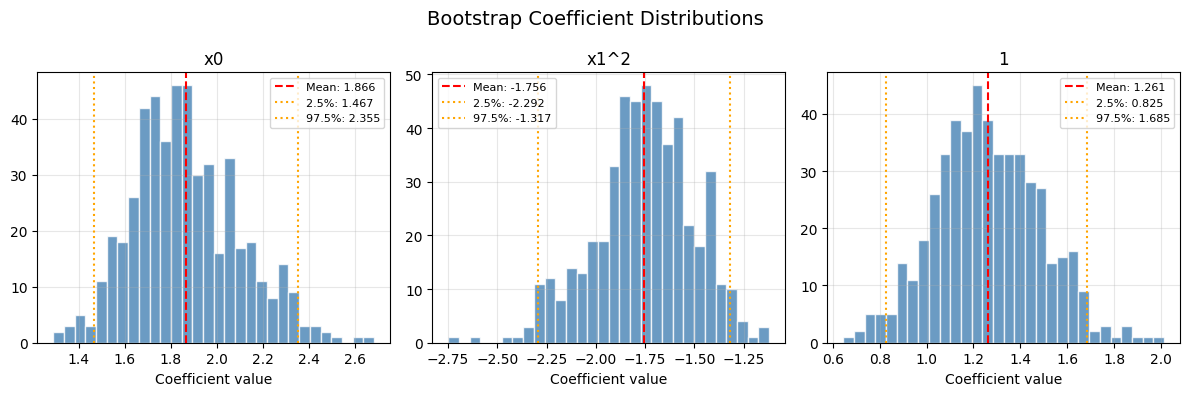
Pairs bootstrap resamples \((X_i, y_i)\) pairs, refits IRLS on each bootstrap sample, and collects coefficient distributions. This gives a nonparametric uncertainty estimate.
boot = bootstrap_classification_coefficients(clf, n_bootstrap=500, alpha=0.05, seed=42)

print("Bootstrap 95% Coefficient Intervals (500 resamples):")
print(f"  {'Term':>15s} {'Mean':>10s} {'Lower':>10s} {'Upper':>10s} {'Std':>10s}")
print("  " + "-" * 55)
for name, mean, lo, hi, std in zip(
    boot["names"],
    boot["mean"],
    boot["lower"],
    boot["upper"],
    boot["std"],
    strict=False,
):
    print(f"  {name:>15s} {float(mean):10.4f} {float(lo):10.4f} {float(hi):10.4f} {float(std):10.4f}")

# Plot bootstrap distributions
n_coefs = boot["coefficients"].shape[1]
fig, axes = plt.subplots(1, n_coefs, figsize=(4 * n_coefs, 4))
if n_coefs == 1:
    axes = [axes]

for i, (ax, name) in enumerate(zip(axes, boot["names"], strict=False)):
    ax.hist(boot["coefficients"][:, i], bins=30, color="steelblue", edgecolor="white", alpha=0.8)
    ax.axvline(float(boot["mean"][i]), color="r", linestyle="--", label=f"Mean: {float(boot['mean'][i]):.3f}")
    ax.axvline(float(boot["lower"][i]), color="orange", linestyle=":", label=f"2.5%: {float(boot['lower'][i]):.3f}")
    ax.axvline(float(boot["upper"][i]), color="orange", linestyle=":", label=f"97.5%: {float(boot['upper'][i]):.3f}")
    ax.set_xlabel("Coefficient value")
    ax.set_title(name)
    ax.legend(fontsize=8)
    ax.grid(True, alpha=0.3)

plt.suptitle("Bootstrap Coefficient Distributions", fontsize=14)
plt.tight_layout()
plt.show()
Bootstrap 95% Coefficient Intervals (500 resamples):
             Term       Mean      Lower      Upper        Std
  -------------------------------------------------------
               x0     1.8660     1.4667     2.3547     0.2314
             x1^2    -1.7561    -2.2923    -1.3175     0.2518
                1     1.2612     0.8245     1.6848     0.2264
Probability calibration#
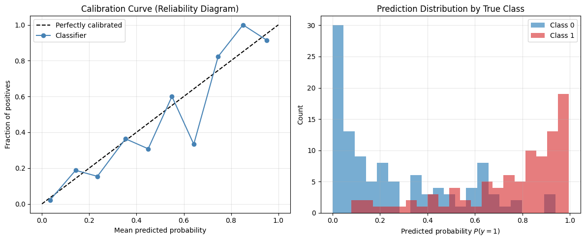
A well-calibrated classifier produces predicted probabilities that match observed frequencies. The reliability diagram (or calibration curve) bins predicted probabilities and compares the average prediction to the actual fraction of positives in each bin.
# Calibration on test data
y_proba_test = np.array(clf.predict_proba(X_test_jax)[:, 1])
y_bin_test = np.array(y_test_jax)

cal = calibration_curve(y_bin_test, y_proba_test, n_bins=10)

fig, axes = plt.subplots(1, 2, figsize=(12, 5))

# Left: reliability diagram
ax = axes[0]
ax.plot([0, 1], [0, 1], "k--", label="Perfectly calibrated")
ax.plot(
    cal["mean_predicted_value"],
    cal["fraction_of_positives"],
    "o-",
    color="steelblue",
    label="Classifier",
)
ax.set_xlabel("Mean predicted probability")
ax.set_ylabel("Fraction of positives")
ax.set_title("Calibration Curve (Reliability Diagram)")
ax.legend()
ax.grid(True, alpha=0.3)

# Right: prediction histogram
ax = axes[1]
ax.hist(y_proba_test[y_bin_test == 0], bins=20, alpha=0.6, label="Class 0", color="tab:blue")
ax.hist(y_proba_test[y_bin_test == 1], bins=20, alpha=0.6, label="Class 1", color="tab:red")
ax.set_xlabel("Predicted probability $P(y=1)$")
ax.set_ylabel("Count")
ax.set_title("Prediction Distribution by True Class")
ax.legend()
ax.grid(True, alpha=0.3)

plt.tight_layout()
plt.show()
Conformal prediction sets#
Conformal prediction provides distribution-free coverage guarantees. Instead of a single predicted class, conformal prediction returns a prediction set — a set of labels guaranteed to contain the true label with probability \(\geq 1 - \alpha\).
The nonconformity score is \(s(x, y) = 1 - P(y \mid x)\): points where the model is uncertain will have larger prediction sets.
# Use test data as calibration, predict on new points
np.random.seed(99)
X_new = np.random.randn(10, 2)
logits_new = 2.0 * X_new[:, 0] - 1.5 * X_new[:, 1] ** 2 + 1.0
probs_new = 1.0 / (1.0 + np.exp(-logits_new))
y_new = (np.random.rand(10) < probs_new).astype(float)

conformal = clf.predict_conformal(
    jnp.array(X_new),
    alpha=0.10,  # 90% coverage
    X_cal=X_test_jax,
    y_cal=y_test_jax,
)

print("Conformal Prediction Sets (90% coverage):")
print(f"  {'Point':>6s}  {'True':>5s}  {'Pred':>5s}  {'P(y=1)':>7s}  Prediction Set")
print("  " + "-" * 50)
proba_new = clf.predict_proba(jnp.array(X_new))
for i in range(len(X_new)):
    pred = int(conformal["y_pred"][i])
    true = int(y_new[i])
    prob = float(proba_new[i, 1])
    pset = conformal["prediction_sets"][i]
    covered = true in pset
    marker = "" if covered else " <-- MISS"
    print(f"  {i:6d}  {true:5d}  {pred:5d}  {prob:7.3f}  {pset}{marker}")
Conformal Prediction Sets (90% coverage):
   Point   True   Pred   P(y=1)  Prediction Set
  --------------------------------------------------
       0      0      0    0.002  {0}
       1      1      0    0.218  {0} <-- MISS
       2      1      1    0.720  {1}
       3      1      1    0.809  {1}
       4      0      0    0.000  {0}
       5      1      1    0.532  {0, 1}
       6      1      1    0.715  {1}
       7      1      0    0.142  {0} <-- MISS
       8      1      1    0.906  {1}
       9      1      0    0.431  {0, 1}
Expression export#
Like SymbolicRegressor, the classifier exports discovered expressions
as SymPy objects, LaTeX strings, or pure NumPy callables. The export
wraps the linear predictor with the sigmoid function.
# SymPy expression (wraps linear predictor with sigmoid)
sympy_expr = clf.to_sympy()
print(f"SymPy expression: {sympy_expr}")

# LaTeX
latex = clf.to_latex()
print(f"\nLaTeX: {latex}")

# Pure NumPy callable
predict_fn = clf.to_callable()
X_demo = np.array([[1.0, 0.0], [0.0, 2.0], [-1.0, -1.0]])
proba_demo = predict_fn(X_demo)

print("\nPure NumPy predictions (no JAX needed):")
for i in range(len(X_demo)):
    print(
        f"  x = {X_demo[i].tolist()} -> "
        f"P(y=0) = {proba_demo[i, 0]:.4f}, P(y=1) = {proba_demo[i, 1]:.4f}"
    )

# Verify callable matches predict_proba
proba_jax = np.array(clf.predict_proba(jnp.array(X_demo)))
print(f"\nMax difference vs predict_proba: {np.max(np.abs(proba_demo - proba_jax)):.2e}")
SymPy expression: 1/(0.290898350314531*exp(-1.82346820831299*x0 + 1.71112668514252*x1**2.0) + 1)

LaTeX: \frac{1}{0.290898350314531 e^{- 1.82346820831299 x_{0} + 1.71112668514252 x_{1}^{2.0}} + 1}
Pure NumPy predictions (no JAX needed):
  x = [1.0, 0.0] -> P(y=0) = 0.0449, P(y=1) = 0.9551
  x = [0.0, 2.0] -> P(y=0) = 0.9964, P(y=1) = 0.0036
  x = [-1.0, -1.0] -> P(y=0) = 0.9089, P(y=1) = 0.0911

Max difference vs predict_proba: 0.00e+00
Multiclass classification#
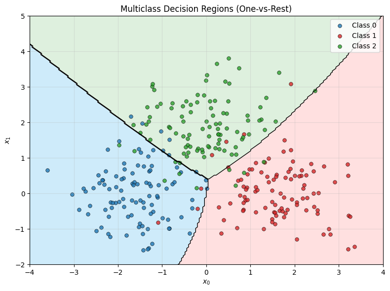
For more than two classes, SymbolicClassifier uses one-vs-rest (OVR).
Each class gets its own binary logistic model with an interpretable
expression. Probabilities are normalized across classes.
We demonstrate this with three clusters that require nonlinear boundaries.
# Generate 3-class data with distinct regions
np.random.seed(42)
n_per_class = 100

# Class 0: centered at (-1.5, 0)
X0 = np.random.randn(n_per_class, 2) * 0.8 + np.array([-1.5, 0])
# Class 1: centered at (1.5, 0)
X1 = np.random.randn(n_per_class, 2) * 0.8 + np.array([1.5, 0])
# Class 2: centered at (0, 2)
X2 = np.random.randn(n_per_class, 2) * 0.8 + np.array([0, 2])

X_mc = np.vstack([X0, X1, X2])
y_mc = np.array([0] * n_per_class + [1] * n_per_class + [2] * n_per_class, dtype=float)

X_mc_jax = jnp.array(X_mc)
y_mc_jax = jnp.array(y_mc)

print(f"Multiclass data: {len(y_mc)} samples, 3 classes ({n_per_class} each)")
Multiclass data: 300 samples, 3 classes (100 each)
# Build library
library_mc = (
    BasisLibrary(n_features=2, feature_names=["x0", "x1"])
    .add_constant()
    .add_linear()
    .add_polynomials(max_degree=2)
    .add_interactions(max_order=2)
)

# Fit multiclass classifier
clf_mc = SymbolicClassifier(
    basis_library=library_mc,
    max_terms=4,
    strategy="greedy_forward",
    information_criterion="bic",
)
clf_mc.fit(X_mc_jax, y_mc_jax)

print(f"Training accuracy: {clf_mc.score(X_mc_jax, y_mc_jax):.4f}\n")

# Print per-class expressions
expressions = clf_mc.expression_
print("Per-class linear predictors (OVR):")
for cls, expr in expressions.items():
    print(f"  Class {cls}: logit = {expr}")
Training accuracy: 0.9133

Per-class linear predictors (OVR):
  Class 0: logit = y = - 3.163*x0 - 0.9921*x1^2 - 1.094*x1
  Class 1: logit = y = 3.551*x0 - 0.4231*x1^2 - 2.063*x1
  Class 2: logit = y = - 1.26*x0^2 + 3.012*x1 - 1.961
# Verify probabilities sum to 1
proba_mc = clf_mc.predict_proba(X_mc_jax)
print(f"Probability matrix shape: {proba_mc.shape}")
print(f"Row sums (should be 1.0): min={float(proba_mc.sum(axis=1).min()):.6f}, "
      f"max={float(proba_mc.sum(axis=1).max()):.6f}")

# Confusion matrix for multiclass
y_pred_mc = clf_mc.predict(X_mc_jax)
cm_mc = compute_confusion_matrix(y_mc_jax, y_pred_mc, n_classes=3)

print("\nConfusion Matrix (Training):")
print(f"  {'':10s}  Pred 0  Pred 1  Pred 2")
for i in range(3):
    print(f"  True {i:4d}  {cm_mc[i, 0]:6d}  {cm_mc[i, 1]:6d}  {cm_mc[i, 2]:6d}")
Probability matrix shape: (300, 3)
Row sums (should be 1.0): min=1.000000, max=1.000000

Confusion Matrix (Training):
              Pred 0  Pred 1  Pred 2
  True    0      93       0       7
  True    1       3      93       4
  True    2       7       5      88
# Plot multiclass decision regions
xx, yy = np.meshgrid(
    np.linspace(-4, 4, 200),
    np.linspace(-2, 5, 200),
)
grid_mc = jnp.array(np.column_stack([xx.ravel(), yy.ravel()]))
pred_grid = np.array(clf_mc.predict(grid_mc)).reshape(xx.shape)

fig, ax = plt.subplots(figsize=(8, 6))
ax.contourf(xx, yy, pred_grid, levels=[-0.5, 0.5, 1.5, 2.5], colors=["#AEDFF7", "#FFCCCC", "#C8E6C9"], alpha=0.6)
ax.contour(xx, yy, pred_grid, levels=[0.5, 1.5], colors="k", linewidths=1)

colors = ["tab:blue", "tab:red", "tab:green"]
for cls in range(3):
    mask = y_mc == cls
    ax.scatter(
        X_mc[mask, 0], X_mc[mask, 1],
        c=colors[cls], edgecolors="k", linewidth=0.5, s=30,
        label=f"Class {cls}", alpha=0.8,
    )

ax.set_xlabel("$x_0$")
ax.set_ylabel("$x_1$")
ax.set_title("Multiclass Decision Regions (One-vs-Rest)")
ax.legend()
ax.grid(True, alpha=0.3)
plt.tight_layout()
plt.show()
Model summary and persistence#
The summary() method prints a comprehensive overview of the fitted model.
Models can be saved to JSON and loaded back for reproducibility.
# Print model summary
print(clf.summary())
============================================================
JAXSR Symbolic Classification Model
============================================================

Type: Binary (classes: [0.0, 1.0])
Linear predictor: y = 1.823*x0 - 1.711*x1^2 + 1.235

Selected terms (3):
  x0: 1.82347
  x1^2: -1.71113
  1: 1.23478

Metrics:
  NLL: 129.6424
  BIC: 276.40
  AIC: 265.28
  Train accuracy: 0.7800
  Log-loss: 0.4321

Training samples: 300
Strategy: greedy_forward
============================================================
import os

# Save and reload
clf.save("classifier_demo.json")
clf_loaded = SymbolicClassifier.load("classifier_demo.json")

# Verify predictions match
proba_orig = np.array(clf.predict_proba(X_jax))
proba_loaded = np.array(clf_loaded.predict_proba(X_jax))
print(f"Max prediction difference after load: {np.max(np.abs(proba_orig - proba_loaded)):.2e}")
print(f"Loaded expression: {clf_loaded.expression_}")

# Clean up
os.remove("classifier_demo.json")
Max prediction difference after load: 0.00e+00
Loaded expression: y = 1.823*x0 - 1.711*x1^2 + 1.235
Convenience function#
For quick exploration, fit_symbolic_classification builds a default
basis library and fits a classifier in one call — analogous to
fit_symbolic for regression.
# Quick classification with convenience function
np.random.seed(42)
X_quick = np.random.randn(200, 2)
y_quick = (X_quick[:, 0] + X_quick[:, 1] > 0).astype(float)

clf_quick = fit_symbolic_classification(
    jnp.array(X_quick),
    jnp.array(y_quick),
    feature_names=["a", "b"],
    max_terms=4,
)

print(f"Discovered: logit = {clf_quick.expression_}")
print(f"Accuracy: {clf_quick.score(jnp.array(X_quick), jnp.array(y_quick)):.4f}")
Discovered: logit = y = 2.16*a
Accuracy: 0.7350
Why did the convenience function miss variable b?
The convenience function fit_symbolic_classification uses default settings: a
small basis library and greedy forward selection. Greedy forward selection adds
one term at a time, choosing whichever single term most improves the information
criterion at each step. Because a alone explains more variance than b alone
(they contribute equally to the true boundary a + b > 0, but the greedy search
commits to one first), the algorithm locks in a and then finds that adding b
does not improve BIC enough given the penalty for an extra parameter at that point.
As a result, the discovered model logit = 2.16*a captures only one of the two
relevant variables and achieves just 73.5% accuracy – well below the 95%+ that
would be achievable with the correct a + b boundary.
For better results on problems like this, build a custom BasisLibrary and use
SymbolicClassifier directly, as demonstrated in the earlier cells of this
notebook. A larger basis library combined with exhaustive search or a less
aggressive information criterion (e.g., AIC instead of BIC) gives the optimizer
more room to discover multi-variable boundaries.
This illustrates the fundamental trade-off of the convenience function: it trades
thoroughness for simplicity. The manual approach – constructing the library,
choosing a strategy, and tuning max_terms – gives you full control over the
search and typically yields better models for non-trivial problems.
Cross-validation#
cross_validate_classification performs k-fold cross-validation,
returning mean and standard deviation of the test score.
from jaxsr import cross_validate_classification

cv_clf = SymbolicClassifier(
    basis_library=library,
    max_terms=5,
    strategy="greedy_forward",
    information_criterion="bic",
)

cv_results = cross_validate_classification(
    cv_clf, X_jax, y_jax, cv=5, scoring="accuracy", random_state=42
)

print("5-Fold Cross-Validation:")
print(f"  Mean accuracy: {cv_results['mean_test_score']:.4f}")
print(f"  Std accuracy:  {cv_results['std_test_score']:.4f}")
print(f"  Fold scores:   {[f'{s:.4f}' for s in cv_results['test_scores']]}")
5-Fold Cross-Validation:
  Mean accuracy: 0.7833
  Std accuracy:  0.0483
  Fold scores:   ['0.7667', '0.8667', '0.7833', '0.7833', '0.7167']
Summary#
Feature |
Method / Property |
|---|---|
Fit a classifier |
|
Predict labels |
|
Predict probabilities |
|
Classification accuracy |
|
All training metrics |
|
Pareto front |
|
Coefficient intervals (Wald) |
|
Conformal prediction sets |
|
Bootstrap coefficients |
|
Calibration curve |
|
Export to SymPy |
|
Export to LaTeX |
|
Export to callable |
|
Save / load |
|
Convenience fit |
|
Cross-validation |
|
Individual metrics |
|