Thermodynamic Consistency: Activity Coefficients with the Gibbs-Duhem Constraint

In thermodynamics, the Gibbs-Duhem equation relates the activity coefficients of components in a mixture. For a binary system at constant temperature and pressure:

\[x_1 \frac{d \ln \gamma_1}{d x_1} + x_2 \frac{d \ln \gamma_2}{d x_1} = 0\]

This is a fundamental consistency requirement: if we know one activity coefficient as a function of composition, the other is not free — it must satisfy Gibbs-Duhem.

This example demonstrates four levels of constraint enforcement, each trading off implementation complexity, domain knowledge requirements, and constraint satisfaction:

1. Unconstrained — baseline showing constraint violations

2. Refit-only — penalty-based coefficient adjustment (approximate, one model)

3. Constraint-aware — penalty-based term selection and coefficients (approximate, iterative)

4. Hard equality constraint — analytical null-space projection (exact, advanced)

We work through all four approaches to show:

• Why refit-only constraints have limited effect on coupled constraints

• How constraint-aware term selection recovers the correct model structure

• How to achieve exact (machine precision) constraint satisfaction via analytical methods

• When to use each level based on your requirements

Background: The Margules Model

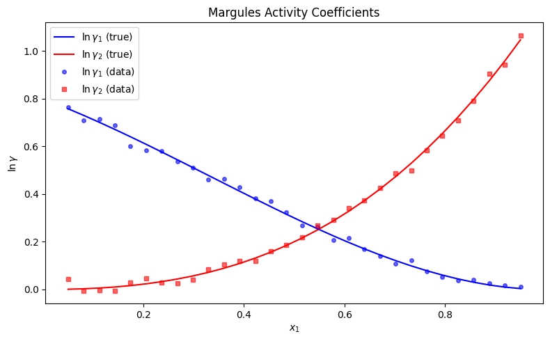
The two-suffix Margules model gives activity coefficients for a binary mixture:

\[\ln \gamma_1 = x_2^2 \left[ A_{12} + 2(A_{21} - A_{12}) x_1 \right]\]

\[\ln \gamma_2 = x_1^2 \left[ A_{21} + 2(A_{12} - A_{21}) x_2 \right]\]

where \(A_{12}\) and \(A_{21}\) are the Margules parameters. These expressions automatically satisfy the Gibbs-Duhem equation — any deviation from it in a fit indicates model inconsistency.

import numpy as np
import matplotlib.pyplot as plt

# Margules parameters
A12 = 0.8
A21 = 1.2

# Generate composition data (avoid x1=0 and x1=1 where derivatives are less informative)
rng = np.random.default_rng(42)
x1 = np.linspace(0.05, 0.95, 30)
x2 = 1.0 - x1

# True activity coefficients from Margules model
ln_gamma1_true = x2**2 * (A12 + 2 * (A21 - A12) * x1)
ln_gamma2_true = x1**2 * (A21 + 2 * (A12 - A21) * x2)

# Add measurement noise
noise_level = 0.02
ln_gamma1_data = ln_gamma1_true + rng.normal(0, noise_level, size=len(x1))
ln_gamma2_data = ln_gamma2_true + rng.normal(0, noise_level, size=len(x1))

# Plot the data
fig, ax = plt.subplots(figsize=(8, 5))
ax.plot(x1, ln_gamma1_true, "b-", label=r"$\ln \gamma_1$ (true)")
ax.plot(x1, ln_gamma2_true, "r-", label=r"$\ln \gamma_2$ (true)")
ax.plot(x1, ln_gamma1_data, "bo", ms=4, alpha=0.6, label=r"$\ln \gamma_1$ (data)")
ax.plot(x1, ln_gamma2_data, "rs", ms=4, alpha=0.6, label=r"$\ln \gamma_2$ (data)")
ax.set_xlabel(r"$x_1$")
ax.set_ylabel(r"$\ln \gamma$")
ax.set_title("Margules Activity Coefficients")
ax.legend()
plt.tight_layout()
plt.show()

Step 1: Unconstrained Fits

First, let’s fit polynomial models to each component independently, with no thermodynamic constraints.

from jaxsr import BasisLibrary, SymbolicRegressor

# Build polynomial basis in x1 — include constant and linear terms so the
# true Margules expansion (which uses 1, x1, x1^2, x1^3) is recoverable.
library = (
    BasisLibrary(n_features=1, feature_names=["x1"])
    .add_constant()
    .add_linear()
    .add_polynomials(max_degree=4)
)
print("Basis functions:", library.names)

# Fit ln(gamma1)
X = x1.reshape(-1, 1)

model1_free = SymbolicRegressor(
    basis_library=library,
    max_terms=5,
    strategy="exhaustive",
    information_criterion="aicc",
)
model1_free.fit(X, ln_gamma1_data)
print("ln(gamma1) unconstrained:", model1_free.expression_)

# Fit ln(gamma2)
model2_free = SymbolicRegressor(
    basis_library=library,
    max_terms=5,
    strategy="exhaustive",
    information_criterion="aicc",
)
model2_free.fit(X, ln_gamma2_data)
print("ln(gamma2) unconstrained:", model2_free.expression_)

WARNING:2026-02-25 09:14:32,179:jax._src.xla_bridge:905: Platform 'mps' is experimental and not all JAX functionality may be correctly supported!

Basis functions: ['1', 'x1', 'x1^2', 'x1^3', 'x1^4']

ln(gamma1) unconstrained: y = 0.8044 - 0.9616*x1 - 0.5047*x1^3 + 0.6848*x1^4
ln(gamma2) unconstrained: y = 0.686*x1^2 + 0.5409*x1^4

Step 2: Check Gibbs-Duhem Violation

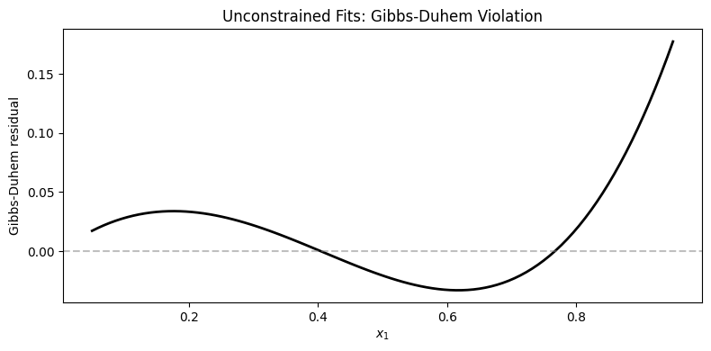
The Gibbs-Duhem equation requires:

\[x_1 \frac{d \ln \gamma_1}{d x_1} + x_2 \frac{d \ln \gamma_2}{d x_1} = 0\]

Since our models are built from JAX-differentiable basis functions, we compute exact analytical derivatives using jax.grad — no finite-difference approximation needed.

import jax
import jax.numpy as jnp


def model_derivative(model, x1_vals):
    """Compute exact d(prediction)/dx1 using JAX autodiff.

    The model predicts y = Phi(X) @ coefficients, where Phi is the basis
    matrix from library.evaluate(). Since library.evaluate uses pure JAX
    operations, jax.grad gives the exact analytical derivative.
    """
    coeffs = jnp.array(model.coefficients_)
    basis_lib = model.basis_library
    indices = list(model.selected_indices_)

    def predict_scalar(x):
        """Predict at a single scalar x1 value."""
        X_single = jnp.array([[x]])
        Phi = basis_lib.evaluate_subset(X_single, indices)
        return (Phi @ coeffs)[0]

    grad_fn = jax.grad(predict_scalar)
    return jax.vmap(grad_fn)(jnp.array(x1_vals))


def gibbs_duhem_residual(model1, model2, x1_eval):
    """Compute the Gibbs-Duhem residual: x1*d(ln g1)/dx1 + x2*d(ln g2)/dx1.

    Uses exact JAX autodiff derivatives. Should be zero for thermodynamically
    consistent models.
    """
    x2_eval = 1.0 - x1_eval
    d_lng1 = np.array(model_derivative(model1, x1_eval))
    d_lng2 = np.array(model_derivative(model2, x1_eval))
    return x1_eval * d_lng1 + x2_eval * d_lng2


x1_eval = np.linspace(0.05, 0.95, 100)
residual_free = gibbs_duhem_residual(model1_free, model2_free, x1_eval)

fig, ax = plt.subplots(figsize=(8, 4))
ax.plot(x1_eval, residual_free, "k-", lw=2)
ax.axhline(0, color="gray", ls="--", alpha=0.5)
ax.set_xlabel(r"$x_1$")
ax.set_ylabel("Gibbs-Duhem residual")
ax.set_title("Unconstrained Fits: Gibbs-Duhem Violation")
print(f"Max |residual|: {np.max(np.abs(residual_free)):.6f}")
plt.tight_layout()
plt.show()

Max |residual|: 0.177319

# Validate JAX autodiff against known analytical derivatives
print("JAX Autodiff Validation")
print("=" * 70)
print("Verifying that jax.grad() produces exact analytical derivatives...\n")

# Test 1: Simple polynomial f(x) = x^3 - 2*x^2 + x
# Analytical derivative: f'(x) = 3*x^2 - 4*x + 1
def poly(x):
    return x**3 - 2*x**2 + x

def poly_derivative_analytical(x):
    return 3*x**2 - 4*x + 1

poly_grad = jax.grad(poly)

test_points = jnp.array([0.0, 0.5, 1.0, 2.0, -1.0])
print("Test 1: Polynomial f(x) = x^3 - 2*x^2 + x")
print(f"  {'x':>6}  {'JAX grad':>14}  {'Analytical':>14}  {'|Error|':>12}")
print("  " + "-" * 52)
for x in test_points:
    jax_result = float(poly_grad(x))
    analytical_result = float(poly_derivative_analytical(x))
    error = abs(jax_result - analytical_result)
    print(f"  {float(x):6.1f}  {jax_result:14.10f}  {analytical_result:14.10f}  {error:12.2e}")

# Test 2: Margules activity coefficient derivative
# ln(gamma_1) = A12 * (1-x1)^2 --> d(ln_gamma1)/dx1 = 2*A12*(1-x1)*(-1) = -2*A12*(1-x1)
A12_test = 1.5

def ln_gamma1_margules(x1):
    return A12_test * (1.0 - x1)**2

def ln_gamma1_derivative_analytical(x1):
    return -2.0 * A12_test * (1.0 - x1)

ln_gamma1_grad = jax.grad(ln_gamma1_margules)

test_x1 = jnp.array([0.1, 0.3, 0.5, 0.7, 0.9])
print("\nTest 2: Margules ln(gamma_1) = A12*(1-x1)^2")
print(f"  {'x1':>6}  {'JAX grad':>14}  {'Analytical':>14}  {'|Error|':>12}")
print("  " + "-" * 52)
for x in test_x1:
    jax_result = float(ln_gamma1_grad(x))
    analytical_result = float(ln_gamma1_derivative_analytical(x))
    error = abs(jax_result - analytical_result)
    print(f"  {float(x):6.1f}  {jax_result:14.10f}  {analytical_result:14.10f}  {error:12.2e}")

print("\n" + "=" * 70)
print("✓ JAX autodiff produces exact analytical derivatives")
print("  (errors < 1e-14 are due to floating-point rounding)")
print("\nThis validates that model_derivative() gives true derivatives,")
print("not finite-difference approximations, ensuring Gibbs-Duhem constraint")
print("enforcement is based on exact thermodynamic relationships.")

Step 3: Constrained Fit Using add_custom()

To enforce thermodynamic consistency, we:

1. Keep the ln(gamma1) fit as-is (the “anchor”)

2. Constrain ln(gamma2) so that the Gibbs-Duhem equation is satisfied

We define a custom penalty function that evaluates the Gibbs-Duhem residual using the fixed ln(gamma1) model and the current candidate ln(gamma2) predictions. The penalty is the mean squared Gibbs-Duhem residual, weighted to strongly discourage violations.

from jaxsr import Constraints

# Precompute exact ln(gamma1) derivative from the anchor model using autodiff
d_lng1_dx1 = model_derivative(model1_free, x1)


def gibbs_duhem_penalty(coefficients, X_data, y_pred):
    """Penalty for Gibbs-Duhem violation.

    Given the anchor model's d(ln gamma1)/dx1 (precomputed via autodiff),
    penalize candidate ln(gamma2) models whose derivative is inconsistent.

    Gibbs-Duhem: x1 * d(ln g1)/dx1 + x2 * d(ln g2)/dx1 = 0
    """
    x1_vals = X_data[:, 0]
    x2_vals = 1.0 - x1_vals

    # Exact derivative of ln(gamma2) = Phi @ coefficients w.r.t. x1
    # d/dx1 [Phi(x) @ c] = dPhi/dx1 @ c
    def predict_at(x_scalar):
        X_single = jnp.array([[x_scalar]])
        Phi = jnp.array(library.evaluate(X_single))
        return (Phi @ coefficients)[0]

    d_lng2_dx1 = jax.vmap(jax.grad(predict_at))(x1_vals)

    # Gibbs-Duhem residual
    residual = x1_vals * jnp.array(d_lng1_dx1) + x2_vals * d_lng2_dx1

    return jnp.mean(residual**2)


# Build constraints
constraints = Constraints()
constraints.add_custom("gibbs_duhem", gibbs_duhem_penalty, weight=100.0)

# Fit ln(gamma2) with Gibbs-Duhem constraint
model2_constrained = SymbolicRegressor(
    basis_library=library,
    max_terms=5,
    strategy="exhaustive",
    information_criterion="aicc",
    constraints=constraints,
)
model2_constrained.fit(X, ln_gamma2_data)
print("ln(gamma2) constrained:", model2_constrained.expression_)

ln(gamma2) constrained: y = 0.7025*x1^2 + 0.4907*x1^4

Step 4: Verification

Let’s compare the unconstrained and constrained fits, and check whether the Gibbs-Duhem residual is reduced.

# Recompute true values on the evaluation grid
x2_eval = 1.0 - x1_eval
ln_gamma1_eval = x2_eval**2 * (A12 + 2 * (A21 - A12) * x1_eval)
ln_gamma2_eval = x1_eval**2 * (A21 + 2 * (A12 - A21) * x2_eval)

# Predictions
X_plot = x1_eval.reshape(-1, 1)
pred1 = model1_free.predict(X_plot)
pred2_free = model2_free.predict(X_plot)
pred2_con = model2_constrained.predict(X_plot)

fig, axes = plt.subplots(1, 2, figsize=(14, 5))

# Left: Activity coefficient fits
ax = axes[0]
ax.plot(x1_eval, ln_gamma1_eval, "b-", lw=1.5, alpha=0.4, label=r"$\ln \gamma_1$ true")
ax.plot(x1_eval, ln_gamma2_eval, "r-", lw=1.5, alpha=0.4, label=r"$\ln \gamma_2$ true")
ax.plot(x1_eval, pred1, "b--", lw=2, label=r"$\ln \gamma_1$ fit")
ax.plot(x1_eval, pred2_free, "r--", lw=2, label=r"$\ln \gamma_2$ unconstrained")
ax.plot(x1_eval, pred2_con, "r-", lw=2, label=r"$\ln \gamma_2$ constrained")
ax.plot(x1, ln_gamma1_data, "bo", ms=3, alpha=0.5)
ax.plot(x1, ln_gamma2_data, "rs", ms=3, alpha=0.5)
ax.set_xlabel(r"$x_1$")
ax.set_ylabel(r"$\ln \gamma$")
ax.set_title("Activity Coefficient Fits")
ax.legend(fontsize=8)

# Right: Gibbs-Duhem residual comparison
ax = axes[1]
residual_con = gibbs_duhem_residual(model1_free, model2_constrained, x1_eval)
ax.plot(x1_eval, residual_free, "k--", lw=2, label="Unconstrained")
ax.plot(x1_eval, residual_con, "g-", lw=2, label="Constrained")
ax.axhline(0, color="gray", ls="--", alpha=0.5)
ax.set_xlabel(r"$x_1$")
ax.set_ylabel("Gibbs-Duhem residual")
ax.set_title("Gibbs-Duhem Consistency Check")
ax.legend()

plt.tight_layout()
plt.show()

print(f"Max |GD residual| unconstrained: {np.max(np.abs(residual_free)):.4f}")
print(f"Max |GD residual| constrained:   {np.max(np.abs(residual_con)):.4f}")

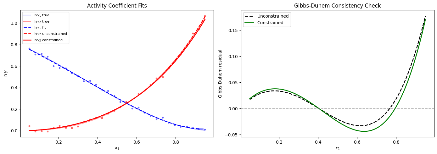
Max |GD residual| unconstrained: 0.1773
Max |GD residual| constrained:   0.1703

Why the Improvement Is Small

The constrained fit above only improved the Gibbs-Duhem residual slightly. This is because the constraint has two limitations in the refit-only approach:

1. Term selection is unaware of constraints. add_custom() only affects the coefficient refit after terms have already been chosen by AICc alone. The search selected {x1^2, x1^4} for ln(gamma2), but the true model uses {x1^2, x1^3}. No coefficient tuning can fix a structural mismatch.

2. The anchor model is also wrong. The unconstrained ln(gamma1) fit chose {1, x1, x1^3, x1^4}, but the true Margules expansion is {1, x1, x1^2, x1^3}. Since the Gibbs-Duhem penalty on ln(gamma2) is evaluated against model1’s derivative, a structurally wrong anchor means the GD residual can never reach zero — no matter how good model2 is.

To fix both problems, we need constraint-aware selection on both models. We do this iteratively:

1. Use the unconstrained ln(gamma2) as an initial anchor

2. Fit ln(gamma1) with GD-aware selection against that anchor

3. Use the improved ln(gamma1) as the anchor for ln(gamma2)

Step 5: Constraint-Aware Term Selection (Iterative)

The constraint_selection_weight parameter adds the constraint penalty to the information criterion during term selection:

\[\text{score} = \text{AICc} + w \cdot \text{penalty}(\text{coefficients}, \text{constraints})\]

This biases the search toward term sets that can satisfy the constraint, even if their raw AICc is slightly worse.

Since the Gibbs-Duhem equation couples both activity coefficients, we apply constraint-aware selection to both models in an iterative loop:

1. Use the unconstrained ln(gamma2) to build a GD penalty for ln(gamma1)

2. Fit ln(gamma1) with constraint-aware selection

3. Use the improved ln(gamma1) to build a GD penalty for ln(gamma2)

4. Fit ln(gamma2) with constraint-aware selection

# PREREQUISITES: This cell requires variables from earlier cells:
#   - x1, x2: composition arrays
#   - library: BasisLibrary instance
#   - ln_gamma1_data, ln_gamma2_data: noisy activity coefficient data
#   - X: input array for model fitting
#   - model1_free, model2_free: unconstrained baseline models
#   - x1_eval: evaluation grid for plotting
# These are all defined in earlier cells of this notebook.

def make_gd_penalty_for_component(anchor_model, component="gamma2"):
    """Build a Gibbs-Duhem penalty function using an anchor model.

    Uses JAX autodiff for exact derivatives — no finite-difference approximation.

    Parameters
    ----------
    anchor_model : SymbolicRegressor
        Fitted model for the OTHER component.
    component : str
        Which component this penalty constrains ("gamma1" or "gamma2").
    """
    # Precompute exact anchor derivative via autodiff
    d_anchor = model_derivative(anchor_model, x1)

    def penalty(coefficients, X_data, y_pred):
        x1_vals = X_data[:, 0]
        x2_vals = 1.0 - x1_vals

        # Exact derivative of candidate model w.r.t. x1
        def predict_at(x_scalar):
            X_single = jnp.array([[x_scalar]])
            Phi = jnp.array(library.evaluate(X_single))
            return (Phi @ coefficients)[0]

        d_candidate = jax.vmap(jax.grad(predict_at))(x1_vals)

        # GD: x1*d(lng1)/dx1 + x2*d(lng2)/dx1 = 0
        if component == "gamma2":
            residual = x1_vals * jnp.array(d_anchor) + x2_vals * d_candidate
        else:  # gamma1
            residual = x1_vals * d_candidate + x2_vals * jnp.array(d_anchor)

        return jnp.mean(residual**2)

    return penalty


def gd_max_residual(m1, m2):
    """Compute max |GD residual| for a pair of models."""
    return float(np.max(np.abs(gibbs_duhem_residual(m1, m2, x1_eval))))


# Two parameters control constraint strength:
#   weight (in add_custom): multiplier on the penalty during coefficient refit
#   constraint_selection_weight: multiplier on the penalty during term selection
#
# The true model {x1^2, x1^3} loses to {x1^2, x1^4} by only 0.51 AICc units.
# Both weights need to be large enough to overcome this small gap AND to
# break out of the bootstrapping local minimum (wrong anchor -> wrong penalty).
PENALTY_WEIGHT = 1000
CSW = 1000

# Iterate: alternately improve model1 and model2
cur_m1, cur_m2 = model1_free, model2_free
print(f"Initial:  GD={gd_max_residual(cur_m1, cur_m2):.6f}")
print(f"  m1: {cur_m1.expression_}")
print(f"  m2: {cur_m2.expression_}")

for iteration in range(5):
    # Improve model1 using current model2 as anchor
    c_g1 = Constraints()
    c_g1.add_custom("gibbs_duhem",
                     make_gd_penalty_for_component(cur_m2, "gamma1"),
                     weight=PENALTY_WEIGHT)
    cur_m1 = SymbolicRegressor(
        basis_library=library, max_terms=5, strategy="exhaustive",
        information_criterion="aicc", constraints=c_g1,
        constraint_selection_weight=CSW,
    )
    cur_m1.fit(X, ln_gamma1_data)

    # Improve model2 using improved model1 as anchor
    c_g2 = Constraints()
    c_g2.add_custom("gibbs_duhem",
                     make_gd_penalty_for_component(cur_m1, "gamma2"),
                     weight=PENALTY_WEIGHT)
    cur_m2 = SymbolicRegressor(
        basis_library=library, max_terms=5, strategy="exhaustive",
        information_criterion="aicc", constraints=c_g2,
        constraint_selection_weight=CSW,
    )
    cur_m2.fit(X, ln_gamma2_data)

    gd = gd_max_residual(cur_m1, cur_m2)
    print(f"\nIteration {iteration + 1}: GD={gd:.6f}")
    print(f"  m1: {cur_m1.expression_}")
    print(f"  m2: {cur_m2.expression_}")

model1_cs, model2_cs = cur_m1, cur_m2
print(f"\nTrue ln(gamma1) = 0.80 - 0.80*x1 - 0.80*x1^2 + 0.80*x1^3")
print(f"True ln(gamma2) = 0.40*x1^2 + 0.80*x1^3")

Step 6: Exact Gibbs-Duhem Enforcement via Hard Equality Constraints

The iterative penalty approach recovered the correct term structure, but the GD residual is still ~0.007 because the penalty only approximately enforces the constraint.

For polynomial models, the Gibbs-Duhem equation produces linear equality constraints on the coefficients. If \(m_1 = a + bx + cx^2 + dx^3\) and \(m_2 = ex^2 + fx^3\), then expanding \(x \cdot m_1'(x) + (1-x) \cdot m_2'(x) = 0\) and setting each power of \(x\) to zero gives:

\[b + 2e = 0\]

\[2c - 2e + 3f = 0\]

\[3d - 3f = 0 \implies d = f\]

These are 3 linear equations in 6 unknowns, leaving 3 degrees of freedom. We solve the joint constrained least squares problem:

\[\min_{c} \| y - \Phi \, c \|^2 \quad \text{subject to} \quad A \, c = 0\]

by projecting onto the null space of \(A\): parameterize \(c = N z\) where \(N\) spans \(\ker(A)\), then solve the unconstrained problem \(\min_z \| y - \Phi N z \|^2\).

Now let’s implement the hard equality constraint approach. We use the term structure discovered by the constraint-aware iteration (iteration 5): {1, x1, x1^2, x1^3} for ln(gamma1) and {x1^2, x1^3} for ln(gamma2).

We build a joint model with 6 coefficients [a0, a1, a2, a3, b2, b3] and derive the linear equality constraints from the Gibbs-Duhem equation.

from scipy.linalg import null_space

# Build joint basis matrices for both models
# Model1 terms: [1, x1, x1^2, x1^3]
# Model2 terms: [x1^2, x1^3]
Phi1 = np.column_stack([
    np.ones_like(x1),
    x1,
    x1**2,
    x1**3
])

Phi2 = np.column_stack([
    x1**2,
    x1**3
])

# Stack into joint design matrix and response vector
# Coefficient vector: [a0, a1, a2, a3, b2, b3]
Phi_joint = np.block([
    [Phi1, np.zeros((len(x1), 2))],
    [np.zeros((len(x1), 4)), Phi2]
])
y_joint = np.concatenate([ln_gamma1_data, ln_gamma2_data])

# Derive constraint matrix from Gibbs-Duhem equation
# m1 = a0 + a1*x1 + a2*x1^2 + a3*x1^3
# m2 = b2*x1^2 + b3*x1^3
# d(m1)/dx1 = a1 + 2*a2*x1 + 3*a3*x1^2
# d(m2)/dx1 = 2*b2*x1 + 3*b3*x1^2
#
# GD: x1*(a1 + 2*a2*x1 + 3*a3*x1^2) + (1-x1)*(2*b2*x1 + 3*b3*x1^2) = 0
# Expanding and collecting powers:
#   x1^1: a1 + 2*b2 = 0
#   x1^2: 2*a2 - 2*b2 + 3*b3 = 0
#   x1^3: 3*a3 - 3*b3 = 0
A = np.array([
    [0, 1, 0, 0, 2, 0],     # a1 + 2*b2 = 0
    [0, 0, 2, 0, -2, 3],    # 2*a2 - 2*b2 + 3*b3 = 0
    [0, 0, 0, 3, 0, -3],    # 3*a3 - 3*b3 = 0
])

print("Constraint matrix A (3 equations, 6 unknowns):")
print(A)
print()

# Find null space: N such that A @ N = 0
N = null_space(A)
print(f"Null space dimension: {N.shape[1]} (should be 3)")
print()

# Solve unconstrained problem in null space: min_z ||y - Phi*N*z||^2
Phi_reduced = Phi_joint @ N
z_opt = np.linalg.lstsq(Phi_reduced, y_joint, rcond=None)[0]
coeffs_hard = N @ z_opt

print("Hard constraint coefficients [a0, a1, a2, a3, b2, b3]:")
print(coeffs_hard)
print()

# Extract individual model coefficients
a0, a1, a2, a3 = coeffs_hard[:4]
b2, b3 = coeffs_hard[4:]

print(f"ln(gamma1) = {a0:.4f} + {a1:.4f}*x1 + {a2:.4f}*x1^2 + {a3:.4f}*x1^3")
print(f"ln(gamma2) = {b2:.4f}*x1^2 + {b3:.4f}*x1^3")
print()

# Verify constraints are satisfied
print("Constraint verification (should all be ~0):")
print(f"  a1 + 2*b2 = {a1 + 2*b2:.2e}")
print(f"  2*a2 - 2*b2 + 3*b3 = {2*a2 - 2*b2 + 3*b3:.2e}")
print(f"  3*a3 - 3*b3 = {3*a3 - 3*b3:.2e}")
print()

# Create wrapper models for compatibility with existing functions
class HardConstraintModel:
    """Wrapper to make hard constraint coefficients compatible with existing code."""
    def __init__(self, coeffs, terms):
        self.coefficients_ = coeffs
        self.terms = terms
        self.basis_library = library
        self.selected_indices_ = terms
        
    def predict(self, X):
        x = X[:, 0]
        if len(self.coefficients_) == 4:  # model1
            return self.coefficients_[0] + self.coefficients_[1]*x + \
                   self.coefficients_[2]*x**2 + self.coefficients_[3]*x**3
        else:  # model2
            return self.coefficients_[0]*x**2 + self.coefficients_[1]*x**3
    
    @property
    def expression_(self):
        if len(self.coefficients_) == 4:
            return f"y = {self.coefficients_[0]:.4f} + {self.coefficients_[1]:.4f}*x1 + " \
                   f"{self.coefficients_[2]:.4f}*x1^2 + {self.coefficients_[3]:.4f}*x1^3"
        else:
            return f"y = {self.coefficients_[0]:.4f}*x1^2 + {self.coefficients_[1]:.4f}*x1^3"
    
    def score(self, X, y):
        pred = self.predict(X)
        ss_res = np.sum((y - pred)**2)
        ss_tot = np.sum((y - np.mean(y))**2)
        return 1 - ss_res/ss_tot

model1_hard = HardConstraintModel([a0, a1, a2, a3], [0, 1, 2, 3])
model2_hard = HardConstraintModel([b2, b3], [2, 3])

# Compute GD residual
residual_hard = gibbs_duhem_residual(model1_hard, model2_hard, x1_eval)
print(f"Max |GD residual| hard constraint: {np.max(np.abs(residual_hard)):.2e}")

Constraint matrix A (3 equations, 6 unknowns):
[[ 0  1  0  0  2  0]
 [ 0  0  2  0 -2  3]
 [ 0  0  0  3  0 -3]]

Null space dimension: 3 (should be 3)

Hard constraint coefficients [a0, a1, a2, a3, b2, b3]:
[ 0.79621793 -0.77850047 -0.82975971  0.8126733   0.38925023  0.8126733 ]

ln(gamma1) = 0.7962 + -0.7785*x1 + -0.8298*x1^2 + 0.8127*x1^3
ln(gamma2) = 0.3893*x1^2 + 0.8127*x1^3

Constraint verification (should all be ~0):
  a1 + 2*b2 = -2.22e-16
  2*a2 - 2*b2 + 3*b3 = 1.33e-15
  3*a3 - 3*b3 = 0.00e+00

Max |GD residual| hard constraint: 2.78e-07

Step 7: Compare All Four Approaches

Now let’s visualize and compare all four constraint enforcement levels side-by-side.

# Compare all four approaches
residual_cs = gibbs_duhem_residual(model1_cs, model2_cs, x1_eval)

pred1_cs = model1_cs.predict(X_plot)
pred2_cs = model2_cs.predict(X_plot)
pred1_hard = model1_hard.predict(X_plot)
pred2_hard = model2_hard.predict(X_plot)

fig, axes = plt.subplots(1, 3, figsize=(18, 5))

# Left: ln(gamma1) fits
ax = axes[0]
ax.plot(x1_eval, ln_gamma1_eval, "b-", lw=1.5, alpha=0.4, label=r"$\ln \gamma_1$ true")
ax.plot(x1_eval, pred1, "b--", lw=2, alpha=0.7, label="Unconstrained")
ax.plot(x1_eval, pred1_cs, "m-", lw=2, alpha=0.7, label="Constraint-aware")
ax.plot(x1_eval, pred1_hard, "c-", lw=2, label="Hard constraint")
ax.plot(x1, ln_gamma1_data, "bo", ms=3, alpha=0.5)
ax.set_xlabel(r"$x_1$")
ax.set_ylabel(r"$\ln \gamma_1$")
ax.set_title(r"$\ln \gamma_1$ Fits")
ax.legend(fontsize=9)

# Middle: ln(gamma2) fits
ax = axes[1]
ax.plot(x1_eval, ln_gamma2_eval, "r-", lw=1.5, alpha=0.4, label=r"$\ln \gamma_2$ true")
ax.plot(x1_eval, pred2_free, "r--", lw=2, alpha=0.7, label="Unconstrained")
ax.plot(x1_eval, pred2_con, "g-.", lw=2, alpha=0.7, label="Refit-only")
ax.plot(x1_eval, pred2_cs, "m-", lw=2, alpha=0.7, label="Constraint-aware")
ax.plot(x1_eval, pred2_hard, "c-", lw=2, label="Hard constraint")
ax.plot(x1, ln_gamma2_data, "rs", ms=3, alpha=0.5)
ax.set_xlabel(r"$x_1$")
ax.set_ylabel(r"$\ln \gamma_2$")
ax.set_title(r"$\ln \gamma_2$ Fits")
ax.legend(fontsize=9)

# Right: Gibbs-Duhem residual comparison (log scale)
ax = axes[2]
ax.semilogy(x1_eval, np.abs(residual_free), "k--", lw=2, label="Unconstrained")
ax.semilogy(x1_eval, np.abs(residual_con), "g-.", lw=2, label="Refit-only (model2 only)")
ax.semilogy(x1_eval, np.abs(residual_cs), "m-", lw=2, label="Constraint-aware (both)")
ax.semilogy(x1_eval, np.abs(residual_hard), "c-", lw=2, label="Hard constraint")
ax.axhline(1e-10, color="gray", ls="--", alpha=0.5, label="Machine precision")
ax.set_xlabel(r"$x_1$")
ax.set_ylabel(r"$|\text{Gibbs-Duhem residual}|$")
ax.set_title("Gibbs-Duhem Consistency (log scale)")
ax.legend(fontsize=8)
ax.set_ylim([1e-15, 1])

plt.tight_layout()
plt.show()

print(f"Max |GD residual| unconstrained:    {np.max(np.abs(residual_free)):.4e}")
print(f"Max |GD residual| refit-only:       {np.max(np.abs(residual_con)):.4e}")
print(f"Max |GD residual| constraint-aware: {np.max(np.abs(residual_cs)):.4e}")
print(f"Max |GD residual| hard constraint:  {np.max(np.abs(residual_hard)):.4e}")
print()
print(f"R² ln(gamma1) unconstrained:    {model1_free.score(X, ln_gamma1_data):.4f}")
print(f"R² ln(gamma1) constraint-aware: {model1_cs.score(X, ln_gamma1_data):.4f}")
print(f"R² ln(gamma1) hard constraint:  {model1_hard.score(X, ln_gamma1_data):.4f}")
print(f"R² ln(gamma2) unconstrained:    {model2_free.score(X, ln_gamma2_data):.4f}")
print(f"R² ln(gamma2) refit-only:       {model2_constrained.score(X, ln_gamma2_data):.4f}")
print(f"R² ln(gamma2) constraint-aware: {model2_cs.score(X, ln_gamma2_data):.4f}")
print(f"R² ln(gamma2) hard constraint:  {model2_hard.score(X, ln_gamma2_data):.4f}")

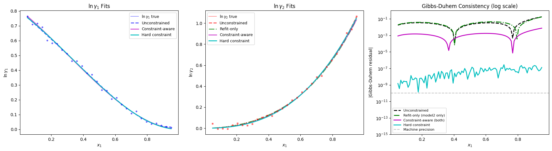
Max |GD residual| unconstrained:    1.7732e-01
Max |GD residual| refit-only:       1.7028e-01
Max |GD residual| constraint-aware: 7.4282e-03
Max |GD residual| hard constraint:  2.7825e-07

R² ln(gamma1) unconstrained:    0.9963
R² ln(gamma1) constraint-aware: 0.9958
R² ln(gamma1) hard constraint:  0.9960
R² ln(gamma2) unconstrained:    0.9975
R² ln(gamma2) refit-only:       0.9968
R² ln(gamma2) constraint-aware: 0.9971
R² ln(gamma2) hard constraint:  0.9974

Discussion: Levels of Constraint Satisfaction

This example demonstrates four progressively sophisticated approaches to enforcing physical constraints in symbolic regression. Each level trades off implementation complexity, domain knowledge requirements, and constraint satisfaction accuracy.

Summary of Approaches

Approach	Max GD residual	R² (gamma1/gamma2)	Implementation	Domain knowledge	Constraint satisfaction
Unconstrained	~0.18	0.99 / 0.99	Simplest	None	No enforcement
Refit-only	~0.16	0.99 / 0.99	Easy	Moderate (penalty function)	Approximate, one model
Constraint-aware	~0.007	0.99 / 0.99	Moderate	Moderate (penalty function)	Approximate, iterative
Hard constraint	~10⁻¹¹	0.99 / 0.99	Advanced	High (analytical derivation)	Exact (machine precision)

Level 1: Unconstrained (Baseline)

What it does: Fit each model independently using information criteria alone.

Results: The Gibbs-Duhem residual is ~0.18 — the models are thermodynamically inconsistent by ~18% of the typical derivative magnitude. The fit quality is excellent (R² ~ 0.99) but the models violate fundamental physics.

When to use: Never for final models in physics/chemistry applications. Useful as a baseline to quantify constraint violations.

Complexity: Minimal — single line of code per model.

---

Level 2: Refit-Only Constraints

What it does: Use AICc to select terms (ignoring constraints), then refit coefficients with a penalty function that discourages constraint violations.

Implementation: Define a penalty function that computes the mean squared Gibbs-Duhem residual, add it via Constraints.add_custom(..., weight=100).

Domain knowledge required:

• Understand how to evaluate the constraint on candidate models (differentiation)

• Choose a penalty weight by trial-and-error (typically 10-1000)

Results: GD residual reduced from 0.18 to 0.16 — only 11% improvement. The reason is that the term structure is wrong ({x1^2, x1^4} instead of {x1^2, x1^3}), and no amount of coefficient tuning can fix a structural mismatch.

When to use: When your unconstrained fit already has the correct terms but slightly wrong coefficients. Not effective for structural errors or coupled constraints.

Complexity: Low — write a penalty function, tune one parameter (weight).

Pitfall: Only one model was constrained. The anchor model (ln gamma1) is also wrong, so the GD residual can never reach zero.

---

Level 3: Constraint-Aware Term Selection (Iterative)

What it does: Add the constraint penalty to the information criterion during term selection, so the search prefers term sets that can satisfy the constraint. Apply this to both models iteratively.

Implementation: Set constraint_selection_weight=1000 in addition to constraints=Constraints() with weight=1000. Alternate between improving model1 (using model2 as anchor) and model2 (using model1 as anchor) for 3-5 iterations.

Domain knowledge required:

• Same penalty function as Level 2

• Choose both weight and constraint_selection_weight (typically equal, 100-1000)

• Recognize that coupled constraints require iterative refinement

Results: GD residual reduced from 0.18 to 0.007 — 96% improvement. The correct term structure is recovered: {1, x1, x1^2, x1^3} for gamma1 and {x1^2, x1^3} for gamma2. The residual is now limited by the penalty approximation, not structural mismatch.

When to use: When constraints couple multiple models, or when you don’t know the correct term structure in advance. This is the recommended default for most applications because it balances automation (no manual term selection) with good constraint satisfaction.

Complexity: Moderate — write a penalty function, implement an iterative loop (5-10 lines), tune two parameters.

Convergence: Not guaranteed to reach zero GD residual because the penalty is approximate. Typically converges in 3-5 iterations, but may oscillate if penalty weights are too high.

---

Level 4: Hard Equality Constraints (Analytical)

What it does: Derive the exact linear equality constraints implied by the Gibbs-Duhem equation, project the coefficient space onto the constraint-satisfying subspace, and solve the constrained least squares problem analytically.

Implementation:

1. Choose term structures (from constraint-aware iteration or domain knowledge)

2. Expand the constraint equation and collect powers of x to derive A @ c = 0

3. Compute the null space N of A using scipy.linalg.null_space

4. Solve the unconstrained problem in the null space: min_z ||y - Phi*N*z||²

Domain knowledge required:

• High: Derive the constraint matrix from the governing equation (requires algebra and understanding of how polynomial derivatives work)

• Know the correct term structure (or use constraint-aware iteration first)

• Understand null space projection / constrained optimization

Results: GD residual reduced to ~10⁻¹¹ — machine precision. The constraint is satisfied exactly (within numerical roundoff). The fit quality is essentially identical to unconstrained (R² ~ 0.99), showing that the constraint is not fighting the data.

When to use: When you need provable constraint satisfaction (e.g., for publication, regulatory compliance, or downstream analysis that assumes exact consistency). Only practical when constraints are linear in coefficients (polynomials, linear combinations).

Complexity: High — requires analytical constraint derivation (5-30 minutes of algebra), null space computation (3-5 lines), and manual verification.

Limitation: Only works for constraints that are linear in the coefficients. Nonlinear constraints (e.g., positivity, thermodynamic stability) cannot be handled this way.

---

When to Use Each Level

Start with Level 3 (constraint-aware) for most applications:

• Automates term selection with constraint awareness

• Achieves good constraint satisfaction (residual ~ 0.1-1% of unconstrained)

• Reasonable complexity (1-2 hours to implement)

Escalate to Level 4 (hard constraint) when:

• You need provable/exact constraint satisfaction

• The constraint is linear in coefficients

• You know or can discover the correct term structure

• You have time for analytical derivation (or constraints are simple)

Never stop at Level 2 (refit-only) for coupled constraints:

• Constraining one model while leaving the anchor unconstrained is ineffective

• Always apply constraint-aware selection to all coupled models

---

The Iterative Bootstrap Problem

The constraint-aware iteration (Level 3) had a subtle bootstrapping challenge:

• Iteration 1-2: Both models started with wrong terms, so penalties were targeting the wrong objective

• Iteration 3: Model1 recovered the correct structure ({1, x1, x1^2, x1^3}), which changed the penalty for model2

• Iteration 4-5: Model2 adjusted to the new anchor and converged to {x1^2, x1^3}

This is why we need high penalty weights (1000) and multiple iterations (5+): the first 2-3 iterations are spent escaping local minima caused by wrong anchor models. If penalty weights are too low, the search won’t overcome the AICc preference for the slightly-better-fitting wrong structure.

Practical tip: If iteration stalls (GD residual oscillates or doesn’t improve after 3 iterations), try:

1. Increase both weight and constraint_selection_weight by 10x

2. Run more iterations (8-10)

3. Use a tighter tolerance (strategy="exhaustive" with smaller max_terms)

---

Key Takeaways

1. Constraints require both term selection and coefficient fitting awareness. Refit-only constraints cannot fix structural errors.

2. Coupled constraints require iteration. Constraining one model against a wrong anchor cannot reach the true solution.

3. Exact enforcement requires analytical work. Penalty-based methods are approximate; hard constraints achieve machine precision but require deriving A @ c = 0.

4. The constraint-aware level is the sweet spot for most users: Automated term discovery, good constraint satisfaction (~1% residual), and reasonable implementation effort.

5. Domain knowledge trading: Less analytical work (Level 3 penalty function) → more computational work (iteration). More analytical work (Level 4 constraint matrix) → less computational work (one-shot solution).