
JAXSR: Comprehensive Tutorial#
This notebook provides a comprehensive introduction to JAXSR, a JAX-based symbolic regression library.
Table of Contents#
1. Installation & Setup#
# Install jaxsr (uncomment if needed)
# !pip install jaxsr

import jax.numpy as jnp
import matplotlib.pyplot as plt
import numpy as np

# Set random seed for reproducibility
np.random.seed(42)

print("Setup complete!")
Setup complete!
2. Basic Usage#
Let’s start with a simple example — discovering the true model:
from jaxsr import BasisLibrary, SymbolicRegressor

# Generate synthetic data
n_samples = 200
X = np.random.randn(n_samples, 2) * 2
y_true = 2.5 * X[:, 0] + 1.2 * X[:, 0] * X[:, 1] - 0.8 * X[:, 1]**2
y = y_true + np.random.randn(n_samples) * 0.1  # Add noise

X_jax = jnp.array(X)
y_jax = jnp.array(y)

print("True model: y = 2.5*x + 1.2*x*y - 0.8*y^2")
print(f"Data shape: X={X.shape}, y={y.shape}")
WARNING:2026-02-25 11:19:43,532:jax._src.xla_bridge:905: Platform 'mps' is experimental and not all JAX functionality may be correctly supported!
True model: y = 2.5*x + 1.2*x*y - 0.8*y^2
Data shape: X=(200, 2), y=(200,)
# Build a basis library
library = (BasisLibrary(n_features=2, feature_names=["x", "y"])
    .add_constant()
    .add_linear()
    .add_polynomials(max_degree=3)
    .add_interactions(max_order=2)
)

print(f"Library contains {len(library)} basis functions:")
print(library.names)
Library contains 8 basis functions:
['1', 'x', 'y', 'x^2', 'x^3', 'y^2', 'y^3', 'x*y']
# Fit the model
model = SymbolicRegressor(
    basis_library=library,
    max_terms=5,
    strategy="greedy_forward",
    information_criterion="bic",
)
model.fit(X_jax, y_jax)

# Results
print("\n" + "="*60)
print("RESULTS")
print("="*60)
print(f"\nDiscovered: {model.expression_}")
print(f"\nR² = {model.metrics_['r2']:.6f}")
print(f"MSE = {model.metrics_['mse']:.6f}")
print(f"BIC = {model.metrics_['bic']:.2f}")
print(f"Complexity = {model.complexity_}")
============================================================
RESULTS
============================================================

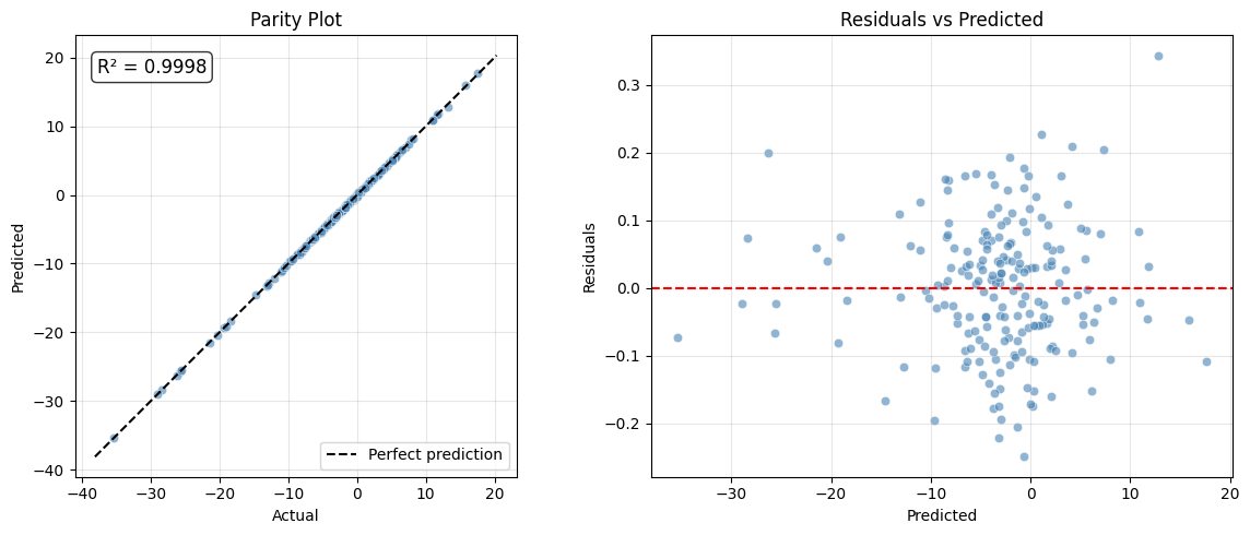
Discovered: y = - 0.7996*y^2 + 2.502*x + 1.198*x*y - 0.002767*x^2

R² = 0.999827
MSE = 0.009535
BIC = -341.78
Complexity = 7
# Parameter significance and diagnostic plots
from scipy import stats as sp_stats

from jaxsr.plotting import plot_parity

intervals = model.coefficient_intervals(alpha=0.05)
n, k = len(y_jax), len(model.selected_features_)
df = n - k

print("Parameter Significance (95% CI):")
print(f"  {'Term':>15s} {'Estimate':>10s} {'Std Err':>9s} {'t':>8s} {'p-value':>10s} 95% CI")
print("  " + "-" * 75)
for name, (est, lo, hi, se) in intervals.items():
    t_val = est / se if abs(se) > 1e-15 else float("inf")
    p_val = float(2 * (1 - sp_stats.t.cdf(abs(t_val), df))) if df > 0 else 0.0
    sig = "***" if p_val < 0.001 else ("**" if p_val < 0.01 else ("*" if p_val < 0.05 else ""))
    print(f"  {name:>15s} {est:10.4f} {se:9.4f} {t_val:8.2f} {p_val:10.2e} [{lo:.4f}, {hi:.4f}] {sig}")
print("  --- *** p<0.001, ** p<0.01, * p<0.05")

# Parity and residual plots
y_pred = model.predict(X_jax)
fig, axes = plt.subplots(1, 2, figsize=(12, 5))
plot_parity(y_jax, y_pred, ax=axes[0], title="Parity Plot")
residuals = np.array(y_jax - y_pred)
axes[1].scatter(np.array(y_pred), residuals, alpha=0.6, c="steelblue", edgecolors="white", linewidth=0.5)
axes[1].axhline(y=0, color="r", linestyle="--")
axes[1].set_xlabel("Predicted")
axes[1].set_ylabel("Residuals")
axes[1].set_title("Residuals vs Predicted")
axes[1].grid(True, alpha=0.3)
plt.tight_layout()
plt.show()
Parameter Significance (95% CI):
             Term   Estimate   Std Err        t    p-value 95% CI
  ---------------------------------------------------------------------------
              y^2    -0.7996    0.0010  -780.22   0.00e+00 [-0.8017, -0.7976] ***
                x     2.5023    0.0037   672.60   0.00e+00 [2.4950, 2.5096] ***
              x*y     1.1983    0.0020   604.49   0.00e+00 [1.1944, 1.2022] ***
              x^2    -0.0028    0.0011    -2.50   1.33e-02 [-0.0049, -0.0006] *
  --- *** p<0.001, ** p<0.01, * p<0.05
# ANOVA table for basic usage fit
from jaxsr import anova

anova_result = anova(model)
summary_sources = {"Model", "Residual", "Total"}

print("ANOVA Table (Basic Usage)")
print("=" * 80)
print(f"  {'Source':25s}  {'DF':>4}  {'Sum Sq':>12}  {'Mean Sq':>12}  {'F':>10}  {'p-value':>10}")
print("-" * 80)
for row in anova_result.rows:
    f_str = f"{row.f_value:10.2f}" if row.f_value is not None else "          "
    p_str = f"{row.p_value:10.4f}" if row.p_value is not None else "          "
    print(f"  {row.source:25s}  {row.df:4d}  {row.sum_sq:12.4f}  {row.mean_sq:12.4f}  {f_str}  {p_str}")
print("-" * 80)

# Percent variance contributions (model terms only)
term_rows = [r for r in anova_result.rows if r.source not in summary_sources]
if term_rows:
    model_ss = sum(r.sum_sq for r in term_rows)
    print("\nVariance Contributions:")
    print("(Percentages relative to Model SS, not Total SS — shows relative importance within fitted model)")
    for row in term_rows:
        pct = 100 * row.sum_sq / model_ss if model_ss > 0 else 0
        sig = (
            "***" if row.p_value is not None and row.p_value < 0.001 else (
            "**" if row.p_value is not None and row.p_value < 0.01 else (
            "*" if row.p_value is not None and row.p_value < 0.05 else ""))
        )
        print(f"  {row.source:25s}  {pct:6.1f}%  {sig}")
# Quick fitting with convenience function
from jaxsr import fit_symbolic

model_quick = fit_symbolic(
    X_jax, y_jax,
    feature_names=["x", "y"],
    max_terms=5,
    max_poly_degree=3,
)

print(f"Quick fit result: {model_quick.expression_}")
/Users/jkitchin/Dropbox/projects/jaxsr/src/jaxsr/regressor.py:1662: UserWarning: Removing 4 basis functions with non-finite values
  return model.fit(X, y)
Quick fit result: y = - 0.7996*y^2 + 2.502*x + 1.198*x*y - 0.002767*x^2
3. Building Basis Libraries#
JAXSR provides flexible ways to build basis libraries with different types of functions.
# Comprehensive library with all function types
comprehensive_library = (BasisLibrary(n_features=2, feature_names=["T", "P"])
    .add_constant()                           # 1
    .add_linear()                             # T, P
    .add_polynomials(max_degree=3)            # T^2, T^3, P^2, P^3
    .add_interactions(max_order=2)            # T*P
    .add_transcendental(["log", "exp", "sqrt", "inv"])  # log(T), exp(T), etc.
    .add_ratios()                             # T/P, P/T
)

print(f"Comprehensive library: {len(comprehensive_library)} functions")
print("\nFunctions:")
for i, name in enumerate(comprehensive_library.names):
    print(f"  [{i:2d}] {name}")
Comprehensive library: 18 functions

Functions:
  [ 0] 1
  [ 1] T
  [ 2] P
  [ 3] T^2
  [ 4] T^3
  [ 5] P^2
  [ 6] P^3
  [ 7] T*P
  [ 8] log(T)
  [ 9] exp(T)
  [10] sqrt(T)
  [11] 1/T
  [12] log(P)
  [13] exp(P)
  [14] sqrt(P)
  [15] 1/P
  [16] T/P
  [17] P/T
# Custom basis functions
custom_library = (BasisLibrary(n_features=2, feature_names=["C_A", "C_B"])
    .add_constant()
    .add_linear()
    .add_custom(
        name="C_A*C_B/(1+C_A)",
        func=lambda X: X[:, 0] * X[:, 1] / (1 + X[:, 0]),
        complexity=4,
    )
    .add_custom(
        name="Arrhenius",
        func=lambda X: jnp.exp(-X[:, 0] / (X[:, 1] + 1e-6)),
        complexity=3,
    )
)

print(f"Custom library: {custom_library.names}")
Custom library: ['1', 'C_A', 'C_B', 'C_A*C_B/(1+C_A)', 'Arrhenius']
# Advanced: Compositions and Rational Forms
advanced_library = (BasisLibrary(n_features=2, feature_names=["x", "y"])
    .add_constant()
    .add_linear()
    .add_compositions(["log", "exp"], ["product", "ratio"])  # log(x*y), exp(x/y)
    .add_rational_forms()  # x/(1+x), x*y/(1+x+y)
    .add_power_laws([0.5, 0.33, 0.67])  # x^0.5, x^(1/3), etc.
)

print(f"Advanced library: {len(advanced_library)} functions")
print("\nSample functions:")
for name in advanced_library.names[:15]:
    print(f"  {name}")
if len(advanced_library.names) > 15:
    print("  ...")
Advanced library: 25 functions

Sample functions:
  1
  x
  y
  log(x*y)
  log(x/y)
  exp(x*y)
  exp(x/y)
  log(y/x)
  exp(y/x)
  x/(1+x)
  x/(1+x)^2
  y/(1+y)
  y/(1+y)^2
  x*y/(1+x)
  x*y/(1+x+y)
  ...
4. Selection Strategies#
JAXSR supports multiple strategies for selecting the best subset of basis functions.
# Generate test data
np.random.seed(42)
X_test = np.random.randn(100, 2)
y_test = 2.0 * X_test[:, 0] - 0.5 * X_test[:, 1]**2 + 1.0

library = (BasisLibrary(n_features=2, feature_names=["x", "y"])
    .add_constant()
    .add_linear()
    .add_polynomials(max_degree=3)
    .add_interactions()
)

X_jax = jnp.array(X_test)
y_jax = jnp.array(y_test)
# Compare different strategies
strategies = ["greedy_forward", "exhaustive"]
results = {}

for strategy in strategies:
    model = SymbolicRegressor(
        basis_library=library,
        max_terms=4,
        strategy=strategy,
    )
    model.fit(X_jax, y_jax)
    results[strategy] = model
    print(f"\n{strategy}:")
    print(f"  Expression: {model.expression_}")
    print(f"  R² = {model.score(X_jax, y_jax):.6f}")
    print(f"  BIC = {model.metrics_['bic']:.2f}")
greedy_forward:
  Expression: y = 2*x + 1 - 0.5*y^2 - 3.5612e-08*y
  R² = 1.000000
  BIC = -2622.28

exhaustive:
  Expression: y = 1 + 2*x - 0.5*y^2
  R² = 1.000000
  BIC = -2583.36
# Explore the Pareto front (complexity vs accuracy tradeoff)
model = results["greedy_forward"]

print("Pareto Front (Complexity vs MSE):")
print("-" * 60)
for result in model.pareto_front_:
    print(f"Complexity {result.complexity:2d} | MSE {result.mse:.6f}")
    print(f"  {result.expression()}")
    print()
Pareto Front (Complexity vs MSE):
------------------------------------------------------------
Complexity  1 | MSE 0.443272
  y = 1.904*x + 0.4944

Complexity  3 | MSE 0.000000
  y = 2*x + 1 - 0.5*y^2

Complexity  4 | MSE 0.000000
  y = 2*x + 1 - 0.5*y^2 - 3.5612e-08*y
5. Regularization#
JAXSR supports L2 (ridge) regularization to prevent overfitting and control coefficient magnitudes.
# Generate noisy data with many potential features
np.random.seed(42)
X_reg = np.random.randn(50, 2)
y_reg = 2.0 * X_reg[:, 0] + 0.5 * X_reg[:, 1] + np.random.randn(50) * 0.5  # More noise

library_large = (BasisLibrary(n_features=2, feature_names=["x", "y"])
    .add_constant()
    .add_linear()
    .add_polynomials(max_degree=4)
    .add_interactions()
)

print(f"Library size: {len(library_large)} functions")
Library size: 10 functions
# Fit without regularization
model_unreg = SymbolicRegressor(
    basis_library=library_large,
    max_terms=5,
    regularization=None,  # No regularization
)
model_unreg.fit(jnp.array(X_reg), jnp.array(y_reg))

print("Without regularization:")
print(f"  Expression: {model_unreg.expression_}")
print(f"  Coefficients: {[float(c) for c in model_unreg.coefficients_]}")
Without regularization:
  Expression: y = 1.943*x + 0.4763*y
  Coefficients: [1.942753553390503, 0.47629597783088684]
6. Physical Constraints#
Incorporate domain knowledge through physical constraints. Here we model a reaction rate with the true form:
from jaxsr import Constraints

# Example: Reaction rate must be non-negative
# and should increase with concentration

# Generate data for a reaction rate
np.random.seed(42)
C = np.random.uniform(0.1, 2.0, 100)
rate = 2.0 * C**0.5  # True: r = 2*sqrt(C)
rate += np.random.randn(100) * 0.05

X = jnp.array(C.reshape(-1, 1))
y = jnp.array(rate)
# Build library
library = (BasisLibrary(n_features=1, feature_names=["C"])
    .add_constant()
    .add_linear()
    .add_polynomials(max_degree=2)
    .add_transcendental(["sqrt", "log"])
)

# Add constraints
constraints = (Constraints()
    .add_bounds("y", lower=0)  # Rate >= 0
    .add_sign_constraint("C", sign="positive")  # Positive coefficient
)

# Fit with constraints
model = SymbolicRegressor(
    basis_library=library,
    max_terms=3,
    constraints=constraints,
)
model.fit(X, y)

print(f"Discovered: {model.expression_}")
print(f"R² = {model.score(X, y):.4f}")
print("\nTrue model: r = 2.0*sqrt(C)")
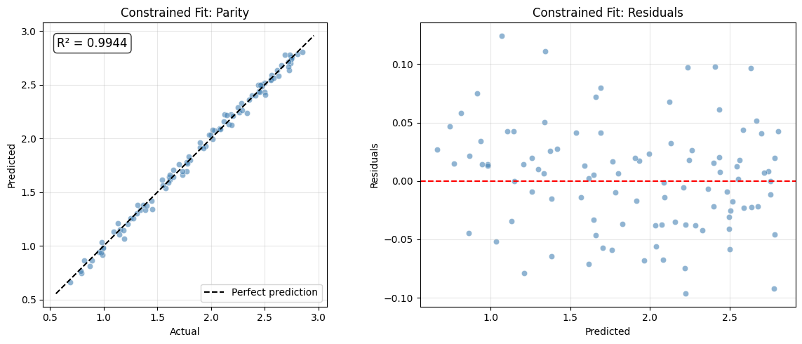
Discovered: y = 1.997*sqrt(C)
R² = 0.9944

True model: r = 2.0*sqrt(C)
# ANOVA table for constrained fit
anova_result = anova(model)
summary_sources = {"Model", "Residual", "Total"}

print("ANOVA Table (Constrained Fit)")
print("=" * 80)
print(f"  {'Source':25s}  {'DF':>4}  {'Sum Sq':>12}  {'Mean Sq':>12}  {'F':>10}  {'p-value':>10}")
print("-" * 80)
for row in anova_result.rows:
    f_str = f"{row.f_value:10.2f}" if row.f_value is not None else "          "
    p_str = f"{row.p_value:10.4f}" if row.p_value is not None else "          "
    print(f"  {row.source:25s}  {row.df:4d}  {row.sum_sq:12.4f}  {row.mean_sq:12.4f}  {f_str}  {p_str}")
print("-" * 80)

term_rows = [r for r in anova_result.rows if r.source not in summary_sources]
if term_rows:
    model_ss = sum(r.sum_sq for r in term_rows)
    print("\nVariance Contributions:")
    print("(Percentages relative to Model SS, not Total SS — shows relative importance within fitted model)")
    for row in term_rows:
        pct = 100 * row.sum_sq / model_ss if model_ss > 0 else 0
        sig = (
            "***" if row.p_value is not None and row.p_value < 0.001 else (
            "**" if row.p_value is not None and row.p_value < 0.01 else (
            "*" if row.p_value is not None and row.p_value < 0.05 else ""))
        )
        print(f"  {row.source:25s}  {pct:6.1f}%  {sig}")
# Parameter significance and diagnostics for constrained fit
from jaxsr.plotting import plot_parity

intervals = model.coefficient_intervals(alpha=0.05)
n_obs, k_terms = len(np.asarray(y)), len(model.selected_features_)
df_resid = n_obs - k_terms

print("Parameter Significance (Constrained Fit):")
print(f"  {'Term':>15s} {'Estimate':>10s} {'Std Err':>9s} {'t':>8s} {'p-value':>10s} 95% CI")
print("  " + "-" * 75)
for name, (est, lo, hi, se) in intervals.items():
    t_val = est / se if abs(se) > 1e-15 else float("inf")
    p_val = float(2 * (1 - sp_stats.t.cdf(abs(t_val), df_resid))) if df_resid > 0 else 0.0
    sig = "***" if p_val < 0.001 else ("**" if p_val < 0.01 else ("*" if p_val < 0.05 else ""))
    print(f"  {name:>15s} {est:10.4f} {se:9.4f} {t_val:8.2f} {p_val:10.2e} [{lo:.4f}, {hi:.4f}] {sig}")
print("  --- *** p<0.001, ** p<0.01, * p<0.05")

# Parity and residual plots
y_pred = model.predict(X)
fig, axes = plt.subplots(1, 2, figsize=(12, 5))
plot_parity(y, y_pred, ax=axes[0], title="Constrained Fit: Parity")
residuals = np.array(y - y_pred)
axes[1].scatter(np.array(y_pred), residuals, alpha=0.6, c="steelblue", edgecolors="white", linewidth=0.5)
axes[1].axhline(y=0, color="r", linestyle="--")
axes[1].set_xlabel("Predicted")
axes[1].set_ylabel("Residuals")
axes[1].set_title("Constrained Fit: Residuals")
axes[1].grid(True, alpha=0.3)
plt.tight_layout()
plt.show()
Parameter Significance (Constrained Fit):
             Term   Estimate   Std Err        t    p-value 95% CI
  ---------------------------------------------------------------------------
          sqrt(C)     1.9975    0.0046   436.81   0.00e+00 [1.9884, 2.0065] ***
  --- *** p<0.001, ** p<0.01, * p<0.05
/var/folders/1f/n8r80n0n5zn2l9h7ghmb94fw0000gn/T/ipykernel_2361/2065125682.py:4: UserWarning: Constraints are active. Classical OLS intervals may not be valid. Consider using bootstrap methods instead.
  intervals = model.coefficient_intervals(alpha=0.05)
# Fixed coefficient example: known intercept
constraints_fixed = (Constraints()
    .add_known_coefficient("1", value=0.0, fixed=True)  # No intercept
)

model_fixed = SymbolicRegressor(
    basis_library=library,
    max_terms=2,
    constraints=constraints_fixed,
)
model_fixed.fit(X, y)

print(f"With fixed intercept=0: {model_fixed.expression_}")
With fixed intercept=0: y = 1.997*sqrt(C)
7. Custom Nonlinear Constraints#
JAXSR supports arbitrary nonlinear constraints through callback functions.
# Example: Constraint that sum of coefficients should be approximately 2.5
def sum_constraint(coeffs, X, y_pred):
    """Penalize if sum of coefficients deviates from 2.5"""
    target_sum = 2.5
    return (jnp.sum(coeffs) - target_sum) ** 2

# Create constraint
custom_constraints = (Constraints()
    .add_custom("sum_equals_2.5", sum_constraint, weight=1.0)
)

print("Created custom constraint: sum of coefficients \u2248 2.5")
Created custom constraint: sum of coefficients ≈ 2.5
# Fit with custom constraint
library_simple = (BasisLibrary(n_features=2, feature_names=["x", "y"])
    .add_constant()
    .add_linear()
    .add_polynomials(max_degree=2)
)

np.random.seed(42)
X_custom = np.random.randn(100, 2)
y_custom = 1.5 * X_custom[:, 0] + 0.8 * X_custom[:, 1] + np.random.randn(100) * 0.1

model_custom = SymbolicRegressor(
    basis_library=library_simple,
    max_terms=3,
    constraints=custom_constraints,
)
model_custom.fit(jnp.array(X_custom), jnp.array(y_custom))

print(f"Expression: {model_custom.expression_}")
print(f"Coefficient sum: {float(jnp.sum(model_custom.coefficients_)):.4f} (target: 2.5)")
Expression: y = 1.597*x + 0.8423*y
Coefficient sum: 2.4396 (target: 2.5)
# Physics constraint: model should pass through a specific point
passthrough_constraints = (Constraints()
    .add_physics_constraint(
        "origin", "passthrough",
        {"point": [0.0, 0.0], "value": 0.0},
        weight=10.0
    )
)

print("Created passthrough constraint: f(0, 0) ≈ 0")
Created passthrough constraint: f(0, 0) ≈ 0
8. Adaptive Sampling#
Iteratively improve models by suggesting new data points to query.
from jaxsr import AdaptiveSampler

# Initial data (sparse)
np.random.seed(42)
X_init = np.random.uniform(0, 5, (20, 2))
y_init = X_init[:, 0]**2 + 2*X_init[:, 1]  # True: y = x^2 + 2y

library = (BasisLibrary(n_features=2, feature_names=["x", "y"])
    .add_constant()
    .add_linear()
    .add_polynomials(max_degree=3)
)

# Initial fit
model = SymbolicRegressor(basis_library=library, max_terms=4)
model.fit(jnp.array(X_init), jnp.array(y_init))

print(f"Initial model: {model.expression_}")
print(f"Initial R² = {model.score(jnp.array(X_init), jnp.array(y_init)):.4f}")
Initial model: y = 1.838*x + 0.1027*y^2 + 0.1398*x^3 + 1.417*y
Initial R² = 0.9969
# Create sampler
sampler = AdaptiveSampler(
    model=model,
    bounds=[(0, 5), (0, 5)],
    strategy="space_filling",
)

# Suggest new points
result = sampler.suggest(n_points=10)
X_new = np.array(result.points)

print(f"\nSuggested {len(X_new)} new points:")
for i, point in enumerate(X_new[:5]):
    print(f"  Point {i+1}: x={point[0]:.2f}, y={point[1]:.2f}")
print("  ...")
Suggested 10 new points:
  Point 1: x=3.18, y=4.84
  Point 2: x=4.99, y=2.06
  Point 3: x=3.56, y=4.72
  Point 4: x=3.93, y=5.00
  Point 5: x=4.98, y=2.69
  ...
# Simulate querying the "oracle" (in practice, run experiments)
y_new = X_new[:, 0]**2 + 2*X_new[:, 1]

# Update model with new data
model.update(jnp.array(X_new), jnp.array(y_new), refit=True)

print(f"\nUpdated model: {model.expression_}")
X_all = np.vstack([X_init, X_new])
y_all = np.concatenate([y_init, y_new])
print(f"Updated R² = {model.score(jnp.array(X_all), jnp.array(y_all)):.4f}")
Updated model: y = 2.191*x + 0.797*y^2 + 0.1245*x^3 - 0.08615*y^3
Updated R² = 0.9986
9. Model Export & Visualization#
# Fit a model
np.random.seed(42)
X = np.random.randn(100, 2)
y = 2.0 * X[:, 0] + X[:, 1]**2 - 0.5

model = fit_symbolic(
    jnp.array(X), jnp.array(y),
    feature_names=["a", "b"],
    max_terms=4,
)

print(f"Expression: {model.expression_}")
Expression: y = 2*a + b^2 - 0.5 - 7.8165e-08*log(a)
# Export to SymPy
try:
    sympy_expr = model.to_sympy()
    print(f"SymPy: {sympy_expr}")

    # LaTeX export
    latex = model.to_latex()
    print(f"LaTeX: {latex}")
except ImportError:
    print("SymPy not available")
SymPy: 1.99999964237213*a + 0.999999761581421*b**2.0 - 7.81645397296415e-8*log(a) - 0.499999672174454
LaTeX: 1.99999964237213 a + 0.999999761581421 b^{2.0} - 7.81645397296415 \cdot 10^{-8} \log{\left(a \right)} - 0.499999672174454
# Export to pure NumPy callable (no JAX dependency)
predict_fn = model.to_callable()

# Use with pure NumPy
X_numpy = np.array([[1.0, 2.0], [3.0, 4.0]])
y_pred = predict_fn(X_numpy)

print(f"NumPy predictions: {y_pred}")
NumPy predictions: [ 5.49999902 21.49999535]
10. Advanced: Chemical Kinetics#
Discover rate laws from kinetic data. The true model follows Langmuir–Hinshelwood kinetics:
# Save and load model
model.save("my_model.json")
loaded_model = SymbolicRegressor.load("my_model.json")

print(f"Loaded model: {loaded_model.expression_}")

# Clean up
import os

os.remove("my_model.json")
Loaded model: y = 2*a + b^2 - 0.5 - 7.8165e-08*log(a)
# Generate Langmuir-Hinshelwood kinetics data
# True: r = k * C_A * C_B / (1 + K * C_A)

np.random.seed(42)
n_samples = 100

C_A = np.random.uniform(0.1, 2.0, n_samples)
C_B = np.random.uniform(0.1, 2.0, n_samples)

k, K = 2.5, 1.2
r_true = k * C_A * C_B / (1 + K * C_A)
r = r_true + np.random.randn(n_samples) * 0.03

X = jnp.column_stack([C_A, C_B])
y = jnp.array(r)

print("True model: r = 2.5*C_A*C_B / (1 + 1.2*C_A)")
True model: r = 2.5*C_A*C_B / (1 + 1.2*C_A)
# Build kinetics-appropriate library
kinetics_library = (BasisLibrary(n_features=2, feature_names=["C_A", "C_B"])
    .add_constant()
    .add_linear()
    .add_interactions(max_order=2)
    .add_rational_forms()  # Langmuir-type terms
    .add_ratios()
)

print(f"Kinetics library: {len(kinetics_library)} functions")
Kinetics library: 16 functions
# Fit with constraint: rate must be non-negative
constraints = Constraints().add_bounds("y", lower=0)

model = SymbolicRegressor(
    basis_library=kinetics_library,
    max_terms=5,
    strategy="greedy_forward",
    constraints=constraints,
)
model.fit(X, y)

print(f"\nDiscovered: {model.expression_}")
print(f"R² = {model.metrics_['r2']:.4f}")
print("\nTrue: r = 2.5*C_A*C_B / (1 + 1.2*C_A)")
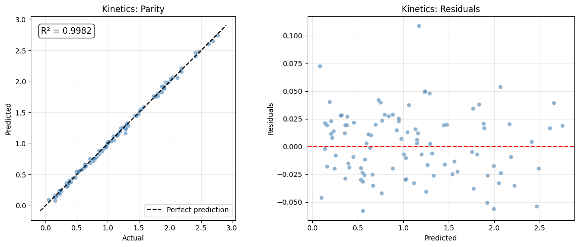
Discovered: y = 2.581*C_A*C_B/(1+C_A) - 0.09397*C_A*C_B - 0.1658*C_A*C_B/(1+C_A+C_B)
R² = 0.9982

True: r = 2.5*C_A*C_B / (1 + 1.2*C_A)
# Parameter significance and diagnostics for kinetics fit
intervals = model.coefficient_intervals(alpha=0.05)
n_obs, k_terms = len(np.asarray(y)), len(model.selected_features_)
df_resid = n_obs - k_terms

print("Parameter Significance (Kinetics Fit):")
print(f"  {'Term':>25s} {'Estimate':>10s} {'Std Err':>9s} {'t':>8s} {'p-value':>10s} 95% CI")
print("  " + "-" * 85)
for name, (est, lo, hi, se) in intervals.items():
    t_val = est / se if abs(se) > 1e-15 else float("inf")
    p_val = float(2 * (1 - sp_stats.t.cdf(abs(t_val), df_resid))) if df_resid > 0 else 0.0
    sig = "***" if p_val < 0.001 else ("**" if p_val < 0.01 else ("*" if p_val < 0.05 else ""))
    print(f"  {name:>25s} {est:10.4f} {se:9.4f} {t_val:8.2f} {p_val:10.2e} [{lo:.4f}, {hi:.4f}] {sig}")
print("  --- *** p<0.001, ** p<0.01, * p<0.05")

# Parity and residual plots
y_pred = model.predict(X)
fig, axes = plt.subplots(1, 2, figsize=(12, 5))
plot_parity(y, y_pred, ax=axes[0], title="Kinetics: Parity")
residuals = np.array(y - y_pred)
axes[1].scatter(np.array(y_pred), residuals, alpha=0.6, c="steelblue", edgecolors="white", linewidth=0.5)
axes[1].axhline(y=0, color="r", linestyle="--")
axes[1].set_xlabel("Predicted")
axes[1].set_ylabel("Residuals")
axes[1].set_title("Kinetics: Residuals")
axes[1].grid(True, alpha=0.3)
plt.tight_layout()
plt.show()
Parameter Significance (Kinetics Fit):
                       Term   Estimate   Std Err        t    p-value 95% CI
  -------------------------------------------------------------------------------------
            C_A*C_B/(1+C_A)     2.5815    0.0353    73.11   0.00e+00 [2.5114, 2.6515] ***
                    C_A*C_B    -0.0940    0.0143    -6.55   2.72e-09 [-0.1224, -0.0655] ***
        C_A*C_B/(1+C_A+C_B)    -0.1658    0.0730    -2.27   2.53e-02 [-0.3106, -0.0210] *
  --- *** p<0.001, ** p<0.01, * p<0.05
/var/folders/1f/n8r80n0n5zn2l9h7ghmb94fw0000gn/T/ipykernel_2361/1242658653.py:2: UserWarning: Constraints are active. Classical OLS intervals may not be valid. Consider using bootstrap methods instead.
  intervals = model.coefficient_intervals(alpha=0.05)
# ANOVA table for kinetics fit
anova_result = anova(model)
summary_sources = {"Model", "Residual", "Total"}

print("ANOVA Table (Kinetics - Langmuir-Hinshelwood)")
print("=" * 80)
print(f"  {'Source':25s}  {'DF':>4}  {'Sum Sq':>12}  {'Mean Sq':>12}  {'F':>10}  {'p-value':>10}")
print("-" * 80)
for row in anova_result.rows:
    f_str = f"{row.f_value:10.2f}" if row.f_value is not None else "          "
    p_str = f"{row.p_value:10.4f}" if row.p_value is not None else "          "
    print(f"  {row.source:25s}  {row.df:4d}  {row.sum_sq:12.4f}  {row.mean_sq:12.4f}  {f_str}  {p_str}")
print("-" * 80)

term_rows = [r for r in anova_result.rows if r.source not in summary_sources]
if term_rows:
    model_ss = sum(r.sum_sq for r in term_rows)
    print("\nVariance Contributions:")
    print("(Percentages relative to Model SS, not Total SS — shows relative importance within fitted model)")
    for row in term_rows:
        pct = 100 * row.sum_sq / model_ss if model_ss > 0 else 0
        sig = (
            "***" if row.p_value is not None and row.p_value < 0.001 else (
            "**" if row.p_value is not None and row.p_value < 0.01 else (
            "*" if row.p_value is not None and row.p_value < 0.05 else ""))
        )
        print(f"  {row.source:25s}  {pct:6.1f}%  {sig}")
11. Advanced: Heat Transfer Correlations#
Discover empirical correlations like Dittus-Boelter.
# Generate Dittus-Boelter correlation data
# True: Nu = 0.023 * Re^0.8 * Pr^0.4

np.random.seed(42)
n_samples = 100

Re = np.random.uniform(10000, 100000, n_samples)
Pr = np.random.uniform(0.7, 100, n_samples)

Nu_true = 0.023 * Re**0.8 * Pr**0.4
Nu = Nu_true * (1 + np.random.randn(n_samples) * 0.03)

# Work in log space
log_Re = np.log(Re)
log_Pr = np.log(Pr)
log_Nu = np.log(Nu)

X = jnp.column_stack([log_Re, log_Pr])
y = jnp.array(log_Nu)

print("True: Nu = 0.023 * Re^0.8 * Pr^0.4")
print(f"Log form: ln(Nu) = {np.log(0.023):.3f} + 0.8*ln(Re) + 0.4*ln(Pr)")
True: Nu = 0.023 * Re^0.8 * Pr^0.4
Log form: ln(Nu) = -3.772 + 0.8*ln(Re) + 0.4*ln(Pr)
# Build heat transfer library and fit in log space
# In log space: ln(Nu) = ln(C) + m*ln(Re) + n*ln(Pr)
ht_library = (BasisLibrary(n_features=2, feature_names=["log_Re", "log_Pr"])
    .add_constant()
    .add_linear()
    .add_interactions(max_order=2)
    .add_polynomials(max_degree=2)
)

ht_model = SymbolicRegressor(
    basis_library=ht_library,
    max_terms=4,
    strategy="greedy_forward",
    information_criterion="bic",
)
ht_model.fit(X, y)

print(f"Discovered (log space): {ht_model.expression_}")
print(f"R² = {ht_model.metrics_['r2']:.6f}")
print(f"\nTrue log-form: ln(Nu) = {np.log(0.023):.3f} + 0.8*ln(Re) + 0.4*ln(Pr)")
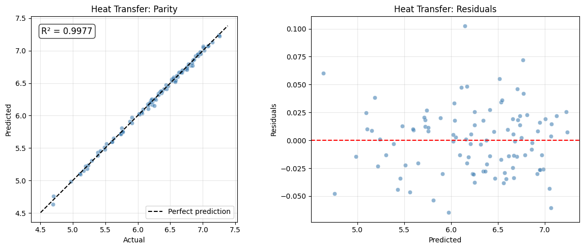
Discovered (log space): y = 0.7787*log_Re + 0.004569*log_Re*log_Pr - 3.558 + 0.3557*log_Pr
R² = 0.997657

True log-form: ln(Nu) = -3.772 + 0.8*ln(Re) + 0.4*ln(Pr)
# ANOVA table for heat transfer fit
ht_anova_result = anova(ht_model)
summary_sources = {"Model", "Residual", "Total"}

print("ANOVA Table (Heat Transfer - Dittus-Boelter)")
print("=" * 80)
print(f"  {'Source':25s}  {'DF':>4}  {'Sum Sq':>12}  {'Mean Sq':>12}  {'F':>10}  {'p-value':>10}")
print("-" * 80)
for row in ht_anova_result.rows:
    f_str = f"{row.f_value:10.2f}" if row.f_value is not None else "          "
    p_str = f"{row.p_value:10.4f}" if row.p_value is not None else "          "
    print(f"  {row.source:25s}  {row.df:4d}  {row.sum_sq:12.4f}  {row.mean_sq:12.4f}  {f_str}  {p_str}")
print("-" * 80)

term_rows = [r for r in ht_anova_result.rows if r.source not in summary_sources]
if term_rows:
    model_ss = sum(r.sum_sq for r in term_rows)
    print("\nVariance Contributions:")
    print("(Percentages relative to Model SS, not Total SS — shows relative importance within fitted model)")
    for row in term_rows:
        pct = 100 * row.sum_sq / model_ss if model_ss > 0 else 0
        sig = (
            "***" if row.p_value is not None and row.p_value < 0.001 else (
            "**" if row.p_value is not None and row.p_value < 0.01 else (
            "*" if row.p_value is not None and row.p_value < 0.05 else ""))
        )
        print(f"  {row.source:25s}  {pct:6.1f}%  {sig}")
# Parameter significance for heat transfer fit
intervals = ht_model.coefficient_intervals(alpha=0.05)
n_obs, k_terms = len(np.asarray(y)), len(ht_model.selected_features_)
df_resid = n_obs - k_terms

print("Parameter Significance (Heat Transfer - Dittus-Boelter):")
print(f"  {'Term':>15s} {'Estimate':>10s} {'Std Err':>9s} {'t':>8s} {'p-value':>10s} 95% CI")
print("  " + "-" * 75)
for name, (est, lo, hi, se) in intervals.items():
    t_val = est / se if abs(se) > 1e-15 else float("inf")
    p_val = float(2 * (1 - sp_stats.t.cdf(abs(t_val), df_resid))) if df_resid > 0 else 0.0
    sig = "***" if p_val < 0.001 else ("**" if p_val < 0.01 else ("*" if p_val < 0.05 else ""))
    print(f"  {name:>15s} {est:10.4f} {se:9.4f} {t_val:8.2f} {p_val:10.2e} [{lo:.4f}, {hi:.4f}] {sig}")
print("  --- *** p<0.001, ** p<0.01, * p<0.05")

# Parity and residual plots
y_pred = ht_model.predict(X)
fig, axes = plt.subplots(1, 2, figsize=(12, 5))
plot_parity(y, y_pred, ax=axes[0], title="Heat Transfer: Parity")
residuals = np.array(y - y_pred)
axes[1].scatter(np.array(y_pred), residuals, alpha=0.6, c="steelblue", edgecolors="white", linewidth=0.5)
axes[1].axhline(y=0, color="r", linestyle="--")
axes[1].set_xlabel("Predicted")
axes[1].set_ylabel("Residuals")
axes[1].set_title("Heat Transfer: Residuals")
axes[1].grid(True, alpha=0.3)
plt.tight_layout()
plt.show()
Parameter Significance (Heat Transfer - Dittus-Boelter):
             Term   Estimate   Std Err        t    p-value 95% CI
  ---------------------------------------------------------------------------
           log_Re     0.7787    0.0235    33.14   0.00e+00 [0.7321, 0.8253] ***
    log_Re*log_Pr     0.0046    0.0063     0.73   4.67e-01 [-0.0079, 0.0170]
                1    -3.5585    0.2513   -14.16   0.00e+00 [-4.0573, -3.0596] ***
           log_Pr     0.3557    0.0669     5.31   6.93e-07 [0.2229, 0.4886] ***
  --- *** p<0.001, ** p<0.01, * p<0.05
# Extract and interpret heat transfer coefficients
print("\nExtracted parameters (log space):")
for name, coef in zip(ht_model.selected_features_, ht_model.coefficients_, strict=False):
    print(f"  {name}: {float(coef):.4f}")

# Recover original Dittus-Boelter form: Nu = C * Re^m * Pr^n
if "1" in ht_model.selected_features_:
    idx = ht_model.selected_features_.index("1")
    ln_C = float(ht_model.coefficients_[idx])
    C = np.exp(ln_C)
    print(f"\nRecovered C = {C:.4f} (true: 0.023)")

if "log_Re" in ht_model.selected_features_:
    idx = ht_model.selected_features_.index("log_Re")
    m = float(ht_model.coefficients_[idx])
    print(f"Recovered Re exponent = {m:.2f} (true: 0.80)")

if "log_Pr" in ht_model.selected_features_:
    idx = ht_model.selected_features_.index("log_Pr")
    n = float(ht_model.coefficients_[idx])
    print(f"Recovered Pr exponent = {n:.2f} (true: 0.40)")
Extracted parameters (log space):
  log_Re: 0.7787
  log_Re*log_Pr: 0.0046
  1: -3.5585
  log_Pr: 0.3557

Recovered C = 0.0285 (true: 0.023)
Recovered Re exponent = 0.78 (true: 0.80)
Recovered Pr exponent = 0.36 (true: 0.40)
12. Uncertainty Quantification#
JAXSR provides comprehensive UQ capabilities. Since models are linear-in-parameters (y = Phi @ beta), classical OLS inference applies directly. JAXSR also supports distribution-free methods (conformal prediction, bootstrap) that make no Gaussian assumption.
Available methods:#
Method |
Assumption |
What it provides |
|---|---|---|
Classical OLS |
Gaussian iid errors |
Coefficient CIs, prediction/confidence bands |
Pareto ensemble |
Multiple models |
Model uncertainty spread |
Bayesian Model Averaging |
IC approximation |
Weighted prediction with between-model variance |
Conformal (jackknife+, split) |
Exchangeability |
Distribution-free coverage guarantee |
Residual bootstrap |
iid residuals |
Non-parametric coefficient/prediction CIs |
# Setup: Generate data with known model and noise level
np.random.seed(42)
n = 150
X_uq = np.random.uniform(0, 5, (n, 1))
y_true_uq = 2.0 * X_uq[:, 0] + 1.0
y_uq = y_true_uq + np.random.randn(n) * 0.5  # Known noise std = 0.5

X_uq_jax = jnp.array(X_uq)
y_uq_jax = jnp.array(y_uq)

# Fit model
library_uq = (BasisLibrary(n_features=1, feature_names=["x"])
    .add_constant()
    .add_linear()
    .add_polynomials(max_degree=3)
)

model_uq = SymbolicRegressor(
    basis_library=library_uq,
    max_terms=3,
    strategy="greedy_forward",
)
model_uq.fit(X_uq_jax, y_uq_jax)

print("True model: y = 2*x + 1  (noise std = 0.5)")
print(f"Discovered: {model_uq.expression_}")
print(f"R² = {model_uq.score(X_uq_jax, y_uq_jax):.4f}")
True model: y = 2*x + 1  (noise std = 0.5)
Discovered: y = 2.017*x + 0.9821
R² = 0.9712
# Noise estimate
print(f"Estimated noise std (sigma): {model_uq.sigma_:.4f}  (true: 0.5)")

# Coefficient confidence intervals
print("\n95% Coefficient Confidence Intervals:")
intervals = model_uq.coefficient_intervals(alpha=0.05)
for name, (est, lo, hi, se) in intervals.items():
    print(f"  {name}: {est:.4f}  [{lo:.4f}, {hi:.4f}]  (SE={se:.4f})")

# Covariance matrix
print("\nCoefficient covariance matrix:")
print(f"  {np.array(model_uq.covariance_matrix_)}")
Estimated noise std (sigma): 0.5170  (true: 0.5)

95% Coefficient Confidence Intervals:
  x: 2.0175  [1.9610, 2.0739]  (SE=0.0286)
  1: 0.9821  [0.8247, 1.1395]  (SE=0.0797)

Coefficient covariance matrix:
  [[ 0.00081609 -0.0019296 ]
 [-0.0019296   0.00634443]]
# Prediction intervals vs confidence bands
X_plot = jnp.linspace(0, 5, 100).reshape(-1, 1)

y_pred, pred_lo, pred_hi = model_uq.predict_interval(X_plot, alpha=0.05)
y_pred_c, conf_lo, conf_hi = model_uq.confidence_band(X_plot, alpha=0.05)

fig, ax = plt.subplots(figsize=(10, 6))
ax.scatter(X_uq[:, 0], y_uq, alpha=0.3, label="Data", color="gray")
ax.plot(X_plot[:, 0], y_pred, "b-", linewidth=2, label="Prediction")
ax.fill_between(X_plot[:, 0], conf_lo, conf_hi, alpha=0.3, color="blue", label="95% Confidence band")
ax.fill_between(X_plot[:, 0], pred_lo, pred_hi, alpha=0.15, color="red", label="95% Prediction interval")
ax.plot(X_plot[:, 0], 2.0 * np.array(X_plot[:, 0]) + 1.0, "k--", alpha=0.5, label="True model")
ax.set_xlabel("x")
ax.set_ylabel("y")
ax.set_title("Classical OLS: Confidence Band vs Prediction Interval")
ax.legend()
plt.tight_layout()
plt.show()

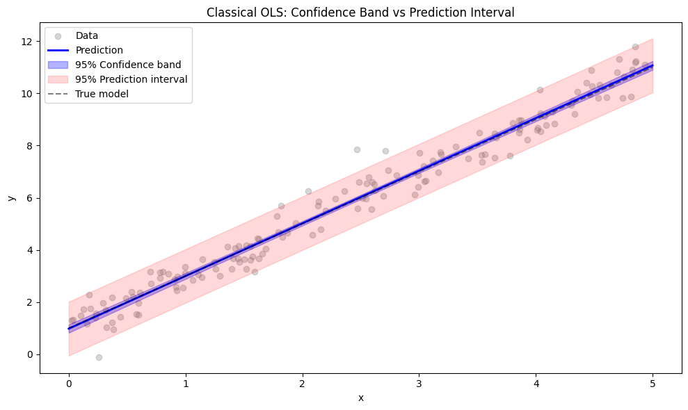
print("Note: Confidence band (blue) estimates E[y|x] — narrower.")
print("      Prediction interval (red) covers a new observation — wider.")
Note: Confidence band (blue) estimates E[y|x] — narrower.
      Prediction interval (red) covers a new observation — wider.
12.2 Pareto Front Ensemble#
The Pareto front contains models at different complexity levels. Ensemble predictions show how much predictions vary across plausible model structures — a measure of model/structural uncertainty.
# Show Pareto front models
print("Pareto front models:")
for r in model_uq.pareto_front_:
    print(f"  Complexity {r.complexity}: {r.expression()}")

# Ensemble predictions
X_new = jnp.linspace(0, 5, 50).reshape(-1, 1)
result = model_uq.predict_ensemble(X_new)

print("\nEnsemble prediction statistics at selected points:")
print(f"  {'x':>5}  {'mean':>8}  {'std':>8}  {'min':>8}  {'max':>8}")
for i in range(0, 50, 10):
    print(
        f"  {float(X_new[i, 0]):5.1f}  "
        f"{float(result['y_mean'][i]):8.3f}  "
        f"{float(result['y_std'][i]):8.3f}  "
        f"{float(result['y_min'][i]):8.3f}  "
        f"{float(result['y_max'][i]):8.3f}"
    )
Pareto front models:
  Complexity 1: y = 2.017*x + 0.9821

Ensemble prediction statistics at selected points:
      x      mean       std       min       max
    0.0     0.982     0.000     0.982     0.982
    1.0     3.041     0.000     3.041     3.041
    2.0     5.099     0.000     5.099     5.099
    3.1     7.158     0.000     7.158     7.158
    4.1     9.217     0.000     9.217     9.217
12.3 Bayesian Model Averaging (BMA)#
BMA weights models by their information criterion: w_k = exp(-0.5 * delta_IC_k) / Z. The BMA variance includes both within-model variance (noise) and between-model variance (model uncertainty).
from jaxsr import BayesianModelAverage

# Create BMA from fitted model
bma = BayesianModelAverage(model_uq, criterion="bic")

print("BMA model weights (BIC-based):")
for expr, weight in bma.weights.items():
    print(f"  {weight:.4f}  {expr}")

# BMA predictions with intervals
y_bma, bma_lo, bma_hi = model_uq.predict_bma(X_plot, criterion="bic", alpha=0.05)

print("\nBMA predictions at selected points:")
print(f"  {'x':>5}  {'pred':>8}  {'lower':>8}  {'upper':>8}")
for i in range(0, 100, 20):
    print(
        f"  {float(X_plot[i, 0]):5.1f}  "
        f"{float(y_bma[i]):8.3f}  "
        f"{float(bma_lo[i]):8.3f}  "
        f"{float(bma_hi[i]):8.3f}"
    )
BMA model weights (BIC-based):
  1.0000  y = 2.017*x + 0.9821

BMA predictions at selected points:
      x      pred     lower     upper
    0.0     0.982    -0.024     1.989
    1.0     3.020     2.013     4.026
    2.0     5.058     4.051     6.064
    3.0     7.096     6.089     8.102
    4.0     9.134     8.127    10.140
12.4 Conformal Prediction#
Distribution-free prediction intervals with finite-sample coverage guarantees. No Gaussian assumption needed.
Jackknife+: Uses LOO residuals from training data (no separate calibration set)
Split conformal: Uses a held-out calibration set
# Jackknife+ conformal prediction (uses training data, no calibration set needed)
X_test_uq = jnp.linspace(0, 5, 50).reshape(-1, 1)
y_test_true = 2.0 * np.array(X_test_uq[:, 0]) + 1.0 + np.random.randn(50) * 0.5

y_conf, conf_lo, conf_hi = model_uq.predict_conformal(
    X_test_uq, alpha=0.10, method="jackknife+"
)

# Check coverage
covered = (y_test_true >= np.array(conf_lo)) & (y_test_true <= np.array(conf_hi))
coverage = np.mean(covered)

print("Jackknife+ conformal prediction (target: 90% coverage):")
print(f"  Actual coverage: {coverage:.1%}")
print(f"  Avg interval width: {float(jnp.mean(conf_hi - conf_lo)):.3f}")

# Split conformal (using held-out calibration data)
X_cal = jnp.array(X_uq[100:])  # Last 50 points as calibration
y_cal = jnp.array(y_uq[100:])

y_conf_s, conf_lo_s, conf_hi_s = model_uq.predict_conformal(
    X_test_uq, alpha=0.10, method="split", X_cal=X_cal, y_cal=y_cal
)

covered_s = (y_test_true >= np.array(conf_lo_s)) & (y_test_true <= np.array(conf_hi_s))
print("\nSplit conformal (target: 90% coverage):")
print(f"  Actual coverage: {np.mean(covered_s):.1%}")
print(f"  Avg interval width: {float(jnp.mean(conf_hi_s - conf_lo_s)):.3f}")
Jackknife+ conformal prediction (target: 90% coverage):
  Actual coverage: 94.0%
  Avg interval width: 1.630

Split conformal (target: 90% coverage):
  Actual coverage: 98.0%
  Avg interval width: 2.037
12.5 Residual Bootstrap#
The residual bootstrap makes no Gaussian assumption. It resamples residuals (y* = y_hat + e*) and refits OLS for each bootstrap sample, giving empirical distributions of coefficients and predictions.
from jaxsr import bootstrap_coefficients, bootstrap_predict

# Bootstrap coefficient CIs
boot_result = bootstrap_coefficients(model_uq, n_bootstrap=2000, alpha=0.05, seed=42)

print("Bootstrap 95% coefficient CIs (B=2000):")
for i, name in enumerate(boot_result["names"]):
    print(
        f"  {name}: {float(boot_result['mean'][i]):.4f} "
        f"[{float(boot_result['lower'][i]):.4f}, {float(boot_result['upper'][i]):.4f}]  "
        f"(std={float(boot_result['std'][i]):.4f})"
    )

# Bootstrap prediction intervals
X_pred = jnp.array([[1.0], [2.5], [4.0]])
boot_pred = bootstrap_predict(model_uq, X_pred, n_bootstrap=2000, alpha=0.05, seed=42)

print("\nBootstrap 95% prediction intervals:")
print(f"  {'x':>5}  {'pred':>8}  {'lower':>8}  {'upper':>8}")
for i in range(len(X_pred)):
    print(
        f"  {float(X_pred[i, 0]):5.1f}  "
        f"{float(boot_pred['y_pred'][i]):8.3f}  "
        f"{float(boot_pred['lower'][i]):8.3f}  "
        f"{float(boot_pred['upper'][i]):8.3f}"
    )
Bootstrap 95% coefficient CIs (B=2000):
  x: 2.0177 [1.9616, 2.0700]  (std=0.0276)
  1: 0.9808 [0.8369, 1.1400]  (std=0.0791)
Bootstrap 95% prediction intervals:
      x      pred     lower     upper
    1.0     3.000     2.891     3.120
    2.5     6.026     5.943     6.112
    4.0     9.052     8.935     9.166
12.6 UQ Visualization#
JAXSR provides built-in plotting functions for UQ: fan charts, coefficient forest plots, and BMA weight charts.
from jaxsr.plotting import (
    plot_bma_weights,
    plot_coefficient_intervals,
    plot_prediction_intervals,
)

fig, axes = plt.subplots(1, 3, figsize=(18, 5))

# Fan chart: prediction intervals (bands from smooth X_plot, data overlaid at actual X_uq)
plot_prediction_intervals(model_uq, X_plot, alpha=0.05, ax=axes[0])
axes[0].scatter(
    np.array(X_uq[:, 0]),
    np.array(y_uq),
    c="black",
    s=20,
    alpha=0.6,
    zorder=5,
    label="Observed",
)
axes[0].legend()
axes[0].set_title("Prediction Intervals Fan Chart")

# Forest plot: coefficient CIs
plot_coefficient_intervals(model_uq, ax=axes[1])
axes[1].set_title("Coefficient Confidence Intervals")

# BMA weights
plot_bma_weights(model_uq, ax=axes[2])
axes[2].set_title("BMA Model Weights (BIC)")

plt.tight_layout()
plt.show()
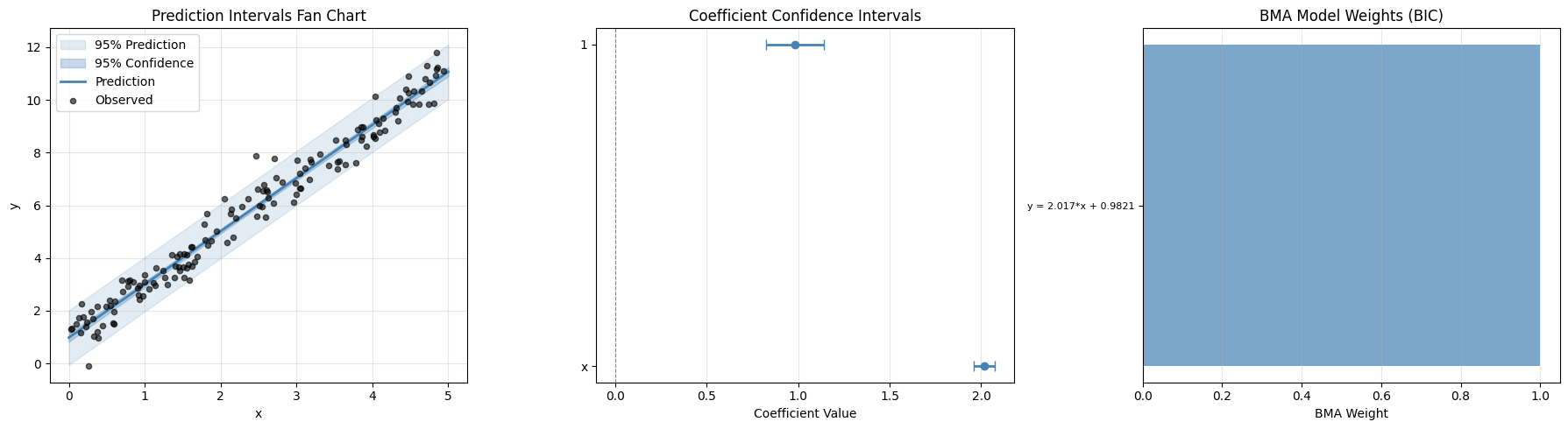
12.7 Comparing UQ Methods#
Different methods answer different questions. Here’s a side-by-side comparison on the same data.
# Compare all UQ methods at specific test points
X_compare = jnp.array([[0.5], [2.5], [4.5]])

# Classical OLS
_, ols_lo, ols_hi = model_uq.predict_interval(X_compare, alpha=0.05)

# BMA
bma_pred, bma_lo, bma_hi = model_uq.predict_bma(X_compare, criterion="bic", alpha=0.05)

# Conformal (jackknife+)
_, conf_lo, conf_hi = model_uq.predict_conformal(X_compare, alpha=0.05, method="jackknife+")

# Bootstrap
boot_result = bootstrap_predict(model_uq, X_compare, n_bootstrap=2000, alpha=0.05, seed=42)

print("Comparison of 95% prediction intervals at x = 0.5, 2.5, 4.5:")
print("=" * 70)
for i, x_val in enumerate([0.5, 2.5, 4.5]):
    print(f"\nx = {x_val}  (true y = {2*x_val + 1:.1f})")
    print(f"  {'Method':<20} {'Lower':>8} {'Upper':>8} {'Width':>8}")
    print(f"  {'-'*20} {'-'*8} {'-'*8} {'-'*8}")

    methods = [
        ("OLS (classical)", float(ols_lo[i]), float(ols_hi[i])),
        ("BMA", float(bma_lo[i]), float(bma_hi[i])),
        ("Conformal (J+)", float(conf_lo[i]), float(conf_hi[i])),
        ("Bootstrap", float(boot_result['lower'][i]), float(boot_result['upper'][i])),
    ]
    for name, lo, hi in methods:
        print(f"  {name:<20} {lo:8.3f} {hi:8.3f} {hi-lo:8.3f}")
Comparison of 95% prediction intervals at x = 0.5, 2.5, 4.5:
======================================================================

x = 0.5  (true y = 2.0)
  Method                  Lower    Upper    Width
  -------------------- -------- -------- --------
  OLS (classical)         0.960    3.021    2.061
  BMA                     0.984    2.997    2.013
  Conformal (J+)          0.955    3.027    2.072
  Bootstrap               1.862    2.128    0.266

x = 2.5  (true y = 6.0)
  Method                  Lower    Upper    Width
  -------------------- -------- -------- --------
  OLS (classical)         5.001    7.051    2.050
  BMA                     5.019    7.032    2.013
  Conformal (J+)          4.990    7.062    2.072
  Bootstrap               5.943    6.112    0.169

x = 4.5  (true y = 10.0)
  Method                  Lower    Upper    Width
  -------------------- -------- -------- --------
  OLS (classical)         9.029   11.093    2.064
  BMA                     9.054   11.067    2.013
  Conformal (J+)          9.025   11.097    2.072
  Bootstrap               9.922   10.193    0.271
Choosing a UQ Method#
When to use |
Method |
|---|---|
Standard case, Gaussian errors |
Classical OLS intervals |
Unknown error distribution |
Conformal prediction or bootstrap |
Multiple plausible models |
Pareto ensemble or BMA |
Need coverage guarantees |
Conformal prediction |
Want coefficient distributions |
Bootstrap |
Constrained/regularized model |
Bootstrap (classical OLS may be invalid) |
Note: When constraints or regularization are active, JAXSR warns that classical OLS intervals may not be valid. Use bootstrap or conformal methods instead.