
Serialization & Sharing: Save, Load, Export, Reproduce#
JAXSR provides multiple serialization formats so you can:
Save and load models, basis libraries, and DOE studies
Share results with collaborators (even those without JAXSR)
Deploy models as pure NumPy callables (no JAX dependency)
Reproduce analyses from saved artifacts
Export equations to LaTeX, SymPy, or callable functions
What Can Be Serialized?#
Object |
Format |
File Extension |
Contains |
|---|---|---|---|
|
JSON |
|
Model expression, coefficients, metrics, basis config |
|
JSON |
|
All basis function definitions (except custom/parametric) |
|
ZIP |
|
Study metadata, designs, observations, fitted model, history |
import json
import os
import atexit
import tempfile

import jax.numpy as jnp
import numpy as np

from jaxsr import BasisLibrary, DOEStudy, SymbolicRegressor, fit_symbolic

np.random.seed(42)

# We'll save everything to a temp directory
SAVE_DIR = tempfile.mkdtemp(prefix="jaxsr_serial_")

# Register cleanup handler to ensure directory is removed even on error
atexit.register(lambda: shutil.rmtree(SAVE_DIR, ignore_errors=True))

print(f"Save directory: {SAVE_DIR}")
1. Saving and Loading Models#
A SymbolicRegressor can be saved to JSON and loaded back with full fidelity —
the loaded model produces identical predictions.
# Fit a model
n = 80
X = np.column_stack([
    np.random.uniform(0, 5, n),
    np.random.uniform(0, 5, n),
])
y = 2.5 * X[:, 0] + 1.2 * X[:, 0] * X[:, 1] - 0.8 * X[:, 1]**2 + 0.3 * np.random.randn(n)

library = (
    BasisLibrary(n_features=2, feature_names=["x1", "x2"])
    .add_constant()
    .add_linear()
    .add_polynomials(max_degree=3)
    .add_interactions(max_order=2)
)

model = SymbolicRegressor(
    basis_library=library, max_terms=5, information_criterion="bic"
)
model.fit(jnp.array(X), jnp.array(y))
print(f"Fitted model: {model.expression_}")
print(f"R² = {model.metrics_['r2']:.6f}")
Fitted model: y = 1.391*x1^2 - 0.06529*x2^3 + 1.092*x1*x2 - 0.1829*x1^3 - 0.4371*x2^2
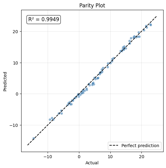
R² = 0.994862
# Quality of fit and parameter significance
import matplotlib.pyplot as plt
from scipy import stats as sp_stats

from jaxsr.plotting import plot_parity

intervals = model.coefficient_intervals(alpha=0.05)
n, k = len(np.asarray(y)), len(model.selected_features_)
df = n - k

print("Parameter Significance (95% CI):")
print(f"  {'Term':>15s} {'Estimate':>10s} {'Std Err':>9s} {'t':>8s} {'p-value':>10s} 95% CI")
print("  " + "-" * 75)
for name, (est, lo, hi, se) in intervals.items():
    t_val = est / se if abs(se) > 1e-15 else float("inf")
    p_val = float(2 * (1 - sp_stats.t.cdf(abs(t_val), df))) if df > 0 else 0.0
    sig = "***" if p_val < 0.001 else ("**" if p_val < 0.01 else ("*" if p_val < 0.05 else ""))
    print(f"  {name:>15s} {est:10.4f} {se:9.4f} {t_val:8.2f} {p_val:10.2e} [{lo:.4f}, {hi:.4f}] {sig}")
print("  --- *** p<0.001, ** p<0.01, * p<0.05")

# Parity plot
y_pred_check = model.predict(jnp.array(X))
fig, ax = plt.subplots(figsize=(6, 6))
plot_parity(jnp.array(y), y_pred_check, ax=ax, title="Parity Plot")
plt.show()
Parameter Significance (95% CI):
             Term   Estimate   Std Err        t    p-value 95% CI
  ---------------------------------------------------------------------------
             x1^2     1.3907    0.0510    27.27   0.00e+00 [1.2891, 1.4922] ***
             x2^3    -0.0653    0.0106    -6.14   3.57e-08 [-0.0865, -0.0441] ***
            x1*x2     1.0915    0.0320    34.09   0.00e+00 [1.0278, 1.1553] ***
             x1^3    -0.1829    0.0108   -16.99   0.00e+00 [-0.2043, -0.1614] ***
             x2^2    -0.4371    0.0480    -9.10   9.66e-14 [-0.5328, -0.3414] ***
  --- *** p<0.001, ** p<0.01, * p<0.05
# ANOVA table for the fitted model
from jaxsr import anova

anova_result = anova(model)

# Filter ANOVA summary rows (Model, Residual, Total) — they are aggregates, not individual terms
summary_sources = {"Model", "Residual", "Total"}

print("ANOVA Table")
print("=" * 80)
print(f"  {'Source':25s}  {'DF':>4}  {'Sum Sq':>12}  {'Mean Sq':>12}  {'F':>10}  {'p-value':>10}")
print("-" * 80)
for row in anova_result.rows:
    f_str = f"{row.f_value:10.2f}" if row.f_value is not None else "          "
    p_str = f"{row.p_value:10.4f}" if row.p_value is not None else "          "
    print(f"  {row.source:25s}  {row.df:4d}  {row.sum_sq:12.4f}  {row.mean_sq:12.4f}  {f_str}  {p_str}")
print("-" * 80)

# Percent variance contributions (model terms only)
# Only compute percentages for individual terms, not summary rows
term_rows = [r for r in anova_result.rows if r.source not in summary_sources]
if term_rows:
    model_ss = sum(r.sum_sq for r in term_rows)
    print("\nVariance Contributions:")
    print("(Percentages relative to Model SS, not Total SS — shows relative importance within fitted model)")
    for row in term_rows:
        pct = 100 * row.sum_sq / model_ss if model_ss > 0 else 0
        sig = (
            "***" if row.p_value is not None and row.p_value < 0.001 else (
            "**" if row.p_value is not None and row.p_value < 0.01 else (
            "*" if row.p_value is not None and row.p_value < 0.05 else ""))
        )
        print(f"  {row.source:25s}  {pct:6.1f}%  {sig}")
# Save the model
model_path = os.path.join(SAVE_DIR, "model.json")
model.save(model_path)
print(f"Model saved to: {model_path}")
print(f"File size: {os.path.getsize(model_path)} bytes")

# Load it back
loaded_model = SymbolicRegressor.load(model_path)
print(f"\nLoaded model: {loaded_model.expression_}")

# Verify predictions match
X_test = np.random.uniform(0, 5, (10, 2))
y_orig = model.predict(jnp.array(X_test))
y_loaded = loaded_model.predict(jnp.array(X_test))
max_diff = float(jnp.max(jnp.abs(y_orig - y_loaded)))
print(f"\nMax prediction difference: {max_diff:.2e}")
assert max_diff < 1e-6, "Predictions should match!"
print("Predictions match perfectly.")
Model saved to: /var/folders/gq/k1kgbl7n539_4dl1md8x3jt80000gn/T/jaxsr_serial_czlrlcmi/model.json
File size: 2830 bytes

Loaded model: y = 1.391*x1^2 - 0.06529*x2^3 + 1.092*x1*x2 - 0.1829*x1^3 - 0.4371*x2^2

Max prediction difference: 0.00e+00
Predictions match perfectly.
# Peek inside the JSON file
with open(model_path) as f:
    data = json.load(f)

print("Model JSON structure:")
print(f"  Top-level keys: {list(data.keys())}")

# The model JSON nests data under 'config', 'basis_library', 'result', etc.
if "result" in data:
    result_keys = list(data["result"].keys())
    print(f"  result keys: {result_keys}")
    print(f"  Selected names: {data['result'].get('selected_names', 'N/A')}")
    print(f"  n_coefficients: {len(data['result'].get('coefficients', []))}")
if "config" in data:
    print(f"  config keys: {list(data['config'].keys())}")
if "basis_library" in data:
    print(f"  basis_library keys: {list(data['basis_library'].keys())}")
Model JSON structure:
  Top-level keys: ['config', 'basis_library', 'result', 'constraints']
  result keys: ['coefficients', 'selected_indices', 'selected_names', 'mse', 'complexity', 'aic', 'bic', 'aicc', 'n_samples']
  Selected names: ['x1^2', 'x2^3', 'x1*x2', 'x1^3', 'x2^2']
  n_coefficients: 5
  config keys: ['max_terms', 'strategy', 'information_criterion', 'cv_folds', 'regularization', 'random_state', 'param_optimizer', 'param_optimization_budget', 'constraint_enforcement']
  basis_library keys: ['n_features', 'feature_names', 'feature_bounds', 'basis_functions']
2. Saving and Loading Basis Libraries#
A BasisLibrary can be saved and loaded independently. This is useful when you
want to reuse the same candidate function set across multiple datasets.
Limitation: Custom functions (add_custom) and parametric functions
(add_parametric) involve Python callables that cannot be serialized.
They raise a ValueError on load and must be re-added manually.
# Create a library
library = (
    BasisLibrary(n_features=3, feature_names=["T", "P", "flow"])
    .add_constant()
    .add_linear()
    .add_polynomials(max_degree=2)
    .add_interactions(max_order=2)
    .add_transcendental(funcs=["log", "exp", "sqrt"])
)
print(f"Library: {len(library)} basis functions")

# Save
lib_path = os.path.join(SAVE_DIR, "basis_library.json")
library.save(lib_path)
print(f"Saved to: {lib_path} ({os.path.getsize(lib_path)} bytes)")

# Load
loaded_lib = BasisLibrary.load(lib_path)
print(f"\nLoaded library: {len(loaded_lib)} basis functions")
print(f"Names match: {library.names == loaded_lib.names}")

# Verify evaluation matches
X_check = np.random.uniform(0.1, 5, (5, 3))
Phi_orig = library.evaluate(jnp.array(X_check))
Phi_loaded = loaded_lib.evaluate(jnp.array(X_check))
max_diff = float(jnp.max(jnp.abs(Phi_orig - Phi_loaded)))
print(f"Max evaluation difference: {max_diff:.2e}")
Library: 19 basis functions
Saved to: /var/folders/gq/k1kgbl7n539_4dl1md8x3jt80000gn/T/jaxsr_serial_czlrlcmi/basis_library.json (4354 bytes)

Loaded library: 19 basis functions
Names match: True
Max evaluation difference: 0.00e+00
3. DOE Study Archives (.jaxsr files)#
A DOEStudy saves everything — metadata, factor definitions, experimental
designs, all observations (with timestamps and notes), and the fitted model —
into a single .jaxsr ZIP archive.
This is the most portable format: share the .jaxsr file and your collaborator
can pick up exactly where you left off.
# Create a study with multiple rounds of data
study = DOEStudy(
    name="heat_exchanger",
    factor_names=["Re", "Pr"],
    bounds=[(5000, 50000), (0.7, 50)],
    description="Nusselt number correlation for heat exchanger design",
)

# Round 1: initial design
X1 = study.create_design(method="latin_hypercube", n_points=15, random_state=42)
y1 = 0.023 * X1[:, 0]**0.8 * X1[:, 1]**0.4 + np.random.randn(15) * 2
study.add_observations(X1, y1, notes="Round 1: initial screening")

# Fit
model = study.fit(max_terms=5)
print(f"Model: {model.expression_}")
print(f"R² = {model.metrics_['r2']:.4f}")

# Round 2: additional data
X2 = np.random.uniform([5000, 0.7], [50000, 50], size=(5, 2))
y2 = 0.023 * X2[:, 0]**0.8 * X2[:, 1]**0.4 + np.random.randn(5) * 2
study.add_observations(X2, y2, notes="Round 2: gap-filling experiments")
model = study.fit(max_terms=5)

# Save
study_path = os.path.join(SAVE_DIR, "heat_exchanger.jaxsr")
study.save(study_path)
print(f"\nStudy saved to: {study_path}")
print(f"File size: {os.path.getsize(study_path)} bytes")
/Users/jkitchin/Dropbox/projects/jaxsr/src/jaxsr/study.py:572: UserWarning: Removing 1 basis functions with non-finite values
  model.fit(self._X_observed, self._y_observed)
Model: y = 0.0001223*Re*Pr + 1.985*sqrt(Re) + 9.404*1/Pr - 24.67*log(Re) + 40.61*log(Pr)
R² = 0.9979
/Users/jkitchin/Dropbox/projects/jaxsr/src/jaxsr/study.py:572: UserWarning: Removing 1 basis functions with non-finite values
  model.fit(self._X_observed, self._y_observed)
Study saved to: /var/folders/gq/k1kgbl7n539_4dl1md8x3jt80000gn/T/jaxsr_serial_czlrlcmi/heat_exchanger.jaxsr
File size: 2565 bytes
# Load the study on a different machine (or in a new session)
loaded_study = DOEStudy.load(study_path)

print(loaded_study.summary())
print(f"\nTotal observations: {loaded_study.n_observations}")
print(f"Is fitted: {loaded_study.is_fitted}")
============================================================
DOE Study: heat_exchanger
============================================================
Description: Nusselt number correlation for heat exchanger design
Factors: Re, Pr
Bounds: [(5000, 50000), (0.7, 50)]

Design: 15 points (15 completed, 0 pending)
Design method: latin_hypercube
Observations: 20

Model: y = 0.0001226*Re*Pr + 2.013*sqrt(Re) + 3.951*1/Pr - 24.5*log(Re) + 38.87*log(Pr)
  MSE: 48.4227
  AIC: 144.3569
  Terms: 5

Iterations: 2
  Round 1: +15 points → y = 0.0001223*Re*Pr + 1.985*sqrt(Re) + 9.404*1/Pr - 24.67*log(Re) + 40.61*log(Pr) (Round 1: initial screening)
  Round 2: +5 points → y = 0.0001226*Re*Pr + 2.013*sqrt(Re) + 3.951*1/Pr - 24.5*log(Re) + 38.87*log(Pr) (Round 2: gap-filling experiments)

Created: 2026-02-10T22:36:54.682536+00:00
Modified: 2026-02-10T22:36:56.353353+00:00
============================================================

Total observations: 20
Is fitted: True
# A collaborator can continue the study: suggest, add data, refit
loaded_study = DOEStudy.load(study_path)

# Suggest next experiments
next_pts = loaded_study.suggest_next(n_points=3, strategy="space_filling")
print("Collaborator's next experiments:")
for i, pt in enumerate(next_pts):
    print(f"  Run {i+1}: Re = {pt[0]:.0f}, Pr = {pt[1]:.2f}")

# They run the experiments and add data
y_new = 0.023 * next_pts[:, 0]**0.8 * next_pts[:, 1]**0.4 + np.random.randn(3) * 2
loaded_study.add_observations(next_pts, y_new, notes="Collaborator round")
loaded_study.fit(max_terms=5)
loaded_study.save(study_path)  # overwrite with updated study

print(f"\nUpdated study: {loaded_study.n_observations} total observations")
Collaborator's next experiments:
  Run 1: Re = 10081, Pr = 0.75
  Run 2: Re = 5815, Pr = 1.05
  Run 3: Re = 5030, Pr = 0.77
/Users/jkitchin/Dropbox/projects/jaxsr/src/jaxsr/study.py:572: UserWarning: Removing 1 basis functions with non-finite values
  model.fit(self._X_observed, self._y_observed)
Updated study: 23 total observations
4. Exporting Models for Deployment#
Once you have a good model, you may want to use it in production without requiring JAX or JAXSR as dependencies.
# Refit our original model
X = np.column_stack([
    np.random.uniform(0, 5, 80),
    np.random.uniform(0, 5, 80),
])
y = 2.5 * X[:, 0] - 0.8 * X[:, 1]**2 + 0.3 * np.random.randn(80)
model = fit_symbolic(jnp.array(X), jnp.array(y), feature_names=["x1", "x2"], max_terms=4)

print(f"Model: {model.expression_}")
print()

# --- Export 1: Pure NumPy callable ---
predict_fn = model.to_callable()

# This function uses only NumPy — no JAX needed
X_new = np.array([[1.0, 2.0], [3.0, 4.0]])
y_pred = predict_fn(X_new)
print(f"NumPy callable predictions: {y_pred}")
print(f"Type: {type(predict_fn)}")
print()

# --- Export 2: SymPy expression ---
sympy_expr = model.to_sympy()
print(f"SymPy: {sympy_expr}")
print(f"Type: {type(sympy_expr)}")
print()

# SymPy enables symbolic manipulation
import sympy

x1, x2 = sympy.symbols("x1 x2")
derivative = sympy.diff(sympy_expr, x1)
print(f"d/dx1: {derivative}")
print()

# --- Export 3: LaTeX ---
latex = model.to_latex()
print(f"LaTeX: ${latex}$")
Model: y = 0.001249*x2^3 + 2.53*x1 - 0.7915*x2^2 - 0.02731*x1*x2

NumPy callable predictions: [-0.68046291 -5.32115615]
Type: <class 'function'>

SymPy: -0.0273054875433445*x1*x2 + 2.5300612449646*x1 - 0.791476964950562*x2**2.0 + 0.00124933442566544*x2**3.0
Type: <class 'sympy.core.add.Add'>

d/dx1: 2.5300612449646 - 0.0273054875433445*x2

LaTeX: $- 0.0273054875433445 x_{1} x_{2} + 2.5300612449646 x_{1} - 0.791476964950562 x_{2}^{2.0} + 0.00124933442566544 x_{2}^{3.0}$
# Deployment pattern: save the callable as a standalone module
# This is how you'd integrate into a production system

deploy_code = f'''\
"""Auto-generated prediction function from JAXSR.

Model: {model.expression_}
R² = {model.metrics_["r2"]:.6f}
Generated with JAXSR v0.1.0
"""
import numpy as np

# Coefficients: {dict(zip(model.selected_features_, [float(c) for c in model.coefficients_], strict=False))}

def predict(X):
    """Predict y from X array of shape (n_samples, 2).

    Features: x1 (column 0), x2 (column 1)
    """
    X = np.asarray(X)
    if X.ndim == 1:
        X = X.reshape(1, -1)
    # Pure NumPy evaluation using exported callable
    # (In production, copy predict_fn code here or import from generated module)
    # For this example, using model.to_callable() which is pure NumPy:
    predict_fn = model.to_callable()  # Replace with inline code in production
    return predict_fn(X)
'''

print("Example deployment module:")
print(deploy_code[:300] + "...")
print()
print("For zero-dependency deployment, use model.to_callable() directly.")
print("The callable is a pure Python/NumPy function with no JAX dependency.")
5. Reproducibility Checklist#
To fully reproduce a JAXSR analysis, save these artifacts:
# Complete reproducibility: save everything
repro_dir = os.path.join(SAVE_DIR, "reproducible")
os.makedirs(repro_dir, exist_ok=True)

# 1. Raw data
np.savez(
    os.path.join(repro_dir, "data.npz"),
    X=X, y=y,
)
print("[1] Saved raw data → data.npz")

# 2. Basis library configuration
library = (
    BasisLibrary(n_features=2, feature_names=["x1", "x2"])
    .add_constant()
    .add_linear()
    .add_polynomials(max_degree=3)
    .add_interactions(max_order=2)
)
library.save(os.path.join(repro_dir, "library.json"))
print("[2] Saved basis library → library.json")

# 3. Fitted model
model.save(os.path.join(repro_dir, "model.json"))
print("[3] Saved fitted model → model.json")

# 4. Metadata
metadata = {
    "jaxsr_version": "0.1.0",
    "random_seed": 42,
    "strategy": "greedy_forward",
    "information_criterion": "bic",
    "max_terms": 4,
    "expression": model.expression_,
    "metrics": {k: float(v) for k, v in model.metrics_.items()},
}
with open(os.path.join(repro_dir, "metadata.json"), "w") as f:
    json.dump(metadata, f, indent=2)
print("[4] Saved metadata → metadata.json")

print(f"\nReproducibility package: {repro_dir}/")
for fname in sorted(os.listdir(repro_dir)):
    size = os.path.getsize(os.path.join(repro_dir, fname))
    print(f"  {fname:25s}  {size:>8} bytes")
[1] Saved raw data → data.npz
[2] Saved basis library → library.json
[3] Saved fitted model → model.json
[4] Saved metadata → metadata.json

Reproducibility package: /var/folders/gq/k1kgbl7n539_4dl1md8x3jt80000gn/T/jaxsr_serial_czlrlcmi/reproducible/
  data.npz                       2410 bytes
  library.json                   1765 bytes
  metadata.json                   385 bytes
  model.json                     4813 bytes
# Reproduce the analysis from saved artifacts
print("Reproducing analysis from saved artifacts...")
print("=" * 50)

# Load data
data = np.load(os.path.join(repro_dir, "data.npz"))
X_repro, y_repro = data["X"], data["y"]

# Load library and refit
lib_repro = BasisLibrary.load(os.path.join(repro_dir, "library.json"))
model_repro = SymbolicRegressor(
    basis_library=lib_repro, max_terms=4, information_criterion="bic"
)
model_repro.fit(jnp.array(X_repro), jnp.array(y_repro))

# Or just load the saved model directly
model_direct = SymbolicRegressor.load(os.path.join(repro_dir, "model.json"))

print(f"Refit model:  {model_repro.expression_}")
print(f"Loaded model: {model_direct.expression_}")
print(f"\nExpressions match: {model_repro.expression_ == model_direct.expression_}")

# Verify predictions
X_test = np.random.uniform(0, 5, (5, 2))
y1 = model_repro.predict(jnp.array(X_test))
y2 = model_direct.predict(jnp.array(X_test))
print(f"Max prediction difference: {float(jnp.max(jnp.abs(y1 - y2))):.2e}")
Reproducing analysis from saved artifacts...
==================================================
Refit model:  y = 0.001249*x2^3 + 2.53*x1 - 0.7915*x2^2 - 0.02731*x1*x2
Loaded model: y = 0.001249*x2^3 + 2.53*x1 - 0.7915*x2^2 - 0.02731*x1*x2

Expressions match: True
Max prediction difference: 0.00e+00
6. What Cannot Be Serialized#
Some objects involve Python callables that cannot be saved to JSON:
Feature |
Serializable? |
Workaround |
|---|---|---|
Standard basis (poly, transcendental) |
Yes |
Reconstructed from config |
Custom basis ( |
No |
Re-add manually after loading |
Parametric basis ( |
No |
Re-add manually after loading |
Constraints |
No |
Reconstruct from code |
Fitted coefficients & metrics |
Yes |
Stored in model JSON |
Pareto front |
Yes |
Stored in model JSON |
For parametric models (like the Langmuir example), save the model JSON for predictions, but keep the fitting script for full reproducibility.
# Clean up temporary files
import os
import shutil

# Add error handling for permission/OS errors
try:
    if os.path.exists(SAVE_DIR):
        shutil.rmtree(SAVE_DIR)
        print(f"✓ Cleaned up: {SAVE_DIR}")
    else:
        print(f"Note: Directory already removed: {SAVE_DIR}")
except PermissionError as e:
    print(f"⚠ Warning: Could not remove {SAVE_DIR} (permission denied)")
    print(f"  You may need to manually delete: {SAVE_DIR}")
except OSError as e:
    print(f"⚠ Warning: Could not remove {SAVE_DIR}")
    print(f"  Error: {e}")
Summary#
Task |
Method |
|---|---|
Save a model |
|
Load a model |
|
Save a basis library |
|
Load a basis library |
|
Save a DOE study |
|
Load a DOE study |
|
Deploy without JAX |
|
Export to SymPy |
|
Export to LaTeX |
|
Best Practices#
For DOE workflows, use
.jaxsrfiles — they capture the entire study lifecycleFor sharing models, use
model.save()— recipients can predict without refittingFor deployment, use
model.to_callable()— zero-dependency NumPy functionFor reproducibility, save data + library + model + metadata together
For publications, use
model.to_latex()andmodel.to_sympy()