ODE Discovery with SINDy-style Sparse Regression

This notebook demonstrates how to discover governing ordinary differential equations (ODEs) from time-series data using JAXSR’s dynamics module. The approach is inspired by SINDy (Sparse Identification of Nonlinear Dynamics), which frames ODE discovery as a sparse regression problem.

The idea: given time-series measurements of state variables \(\mathbf{X}(t)\), we:

1. Estimate derivatives \(\dot{\mathbf{X}} = d\mathbf{X}/dt\) from the data

2. Build a library of candidate nonlinear functions of \(\mathbf{X}\)

3. Fit a sparse model \(\dot{x}_i = \Theta(\mathbf{X})\,\boldsymbol{\xi}_i\) for each state variable

JAXSR wraps this workflow in three functions:

• estimate_derivatives() — numerical differentiation (finite difference, Savitzky-Golay, or spline)

• discover_dynamics() — end-to-end ODE discovery

• DynamicsResult — result container with models, equations, and metrics

import matplotlib.pyplot as plt
import numpy as np
from scipy.integrate import solve_ivp

from jaxsr import BasisLibrary, discover_dynamics, estimate_derivatives

1. Exponential Decay: A Single ODE

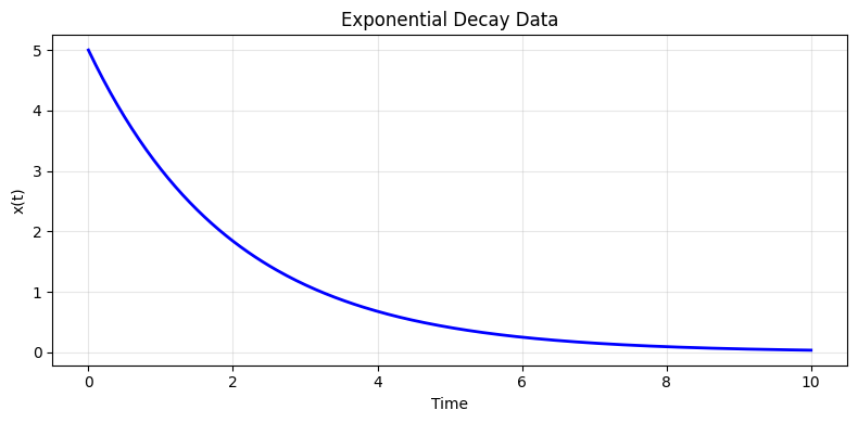
The simplest test case. The true system is:

\[\frac{dx}{dt} = -0.5\,x, \qquad x(0) = 5\]

The exact solution is \(x(t) = 5\,e^{-0.5t}\).

# Generate clean data from the exact solution
t_decay = np.linspace(0, 10, 300)
X_decay = (5.0 * np.exp(-0.5 * t_decay)).reshape(-1, 1)

fig, ax = plt.subplots(figsize=(8, 4))
ax.plot(t_decay, X_decay, "b-", linewidth=2)
ax.set_xlabel("Time")
ax.set_ylabel("x(t)")
ax.set_title("Exponential Decay Data")
ax.grid(True, alpha=0.3)
plt.tight_layout()
plt.show()

result_decay = discover_dynamics(
    X_decay,
    t_decay,
    state_names=["x"],
    max_terms=3,
    strategy="greedy_forward",
    information_criterion="bic",
)

print(result_decay.summary())

Discovered ODEs
========================================
d(x)/dt = y = - 0.4993*x + 0.0001528*x^3 - 0.0007652*x^2
  R² = 1.0000, MSE = 1.19e-06, AIC = -3234.7, BIC = -3223.6

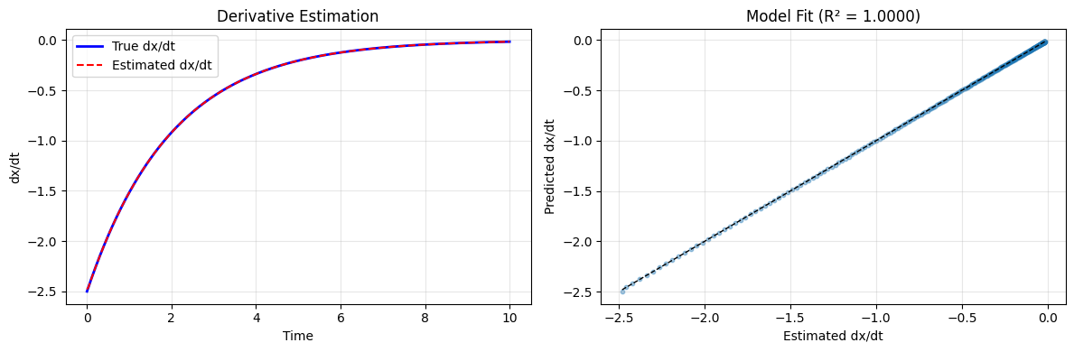
Note on spurious terms: The discovered equation dx/dt = -0.4993*x + 0.0001528*x^3 - 0.0007652*x^2 includes two extra terms beyond the true dynamics dx/dt = -0.5*x. However:

• The dominant term -0.4993*x recovers the true coefficient to within 0.1%, correctly capturing the exponential decay dynamics.

• The spurious x^3 and x^2 terms have negligible coefficients (|coeff| < 0.001), roughly three orders of magnitude smaller than the true coefficient. They do not materially affect trajectory predictions.

• Why does this happen? Greedy forward selection with BIC can over-select terms when spurious coefficients are small but non-zero due to finite data and numerical derivative estimation. BIC’s log(n) penalty was insufficient to offset the marginal improvement in fit from these nearly-zero terms.

• Practical remedies: (1) Apply post-hoc coefficient thresholding – terms with |coefficient| < noise_level / max_basis_value should be treated as spurious and removed. (2) Use a stricter information criterion or increase the penalty weight. (3) Inspect coefficient magnitudes and retain only those consistent with the expected signal-to-noise ratio.

# Compare estimated vs true derivatives
dxdt_true = -0.5 * X_decay[:, 0]

fig, axes = plt.subplots(1, 2, figsize=(12, 4))

axes[0].plot(t_decay, dxdt_true, "b-", label="True dx/dt", linewidth=2)
axes[0].plot(t_decay, result_decay.derivatives[:, 0], "r--", label="Estimated dx/dt", linewidth=1.5)
axes[0].set_xlabel("Time")
axes[0].set_ylabel("dx/dt")
axes[0].set_title("Derivative Estimation")
axes[0].legend()
axes[0].grid(True, alpha=0.3)

# Parity plot: predicted vs estimated derivatives
model_x = result_decay.models["x"]
dxdt_pred = np.asarray(model_x.predict(X_decay))
axes[1].scatter(result_decay.derivatives[:, 0], dxdt_pred, alpha=0.4, s=10)
lims = [result_decay.derivatives[:, 0].min(), result_decay.derivatives[:, 0].max()]
axes[1].plot(lims, lims, "k--", linewidth=1)
axes[1].set_xlabel("Estimated dx/dt")
axes[1].set_ylabel("Predicted dx/dt")
axes[1].set_title(f"Model Fit (R\u00b2 = {result_decay.metrics['x']['r2']:.4f})")
axes[1].grid(True, alpha=0.3)

plt.tight_layout()
plt.show()

2. Comparing Derivative Estimation Methods

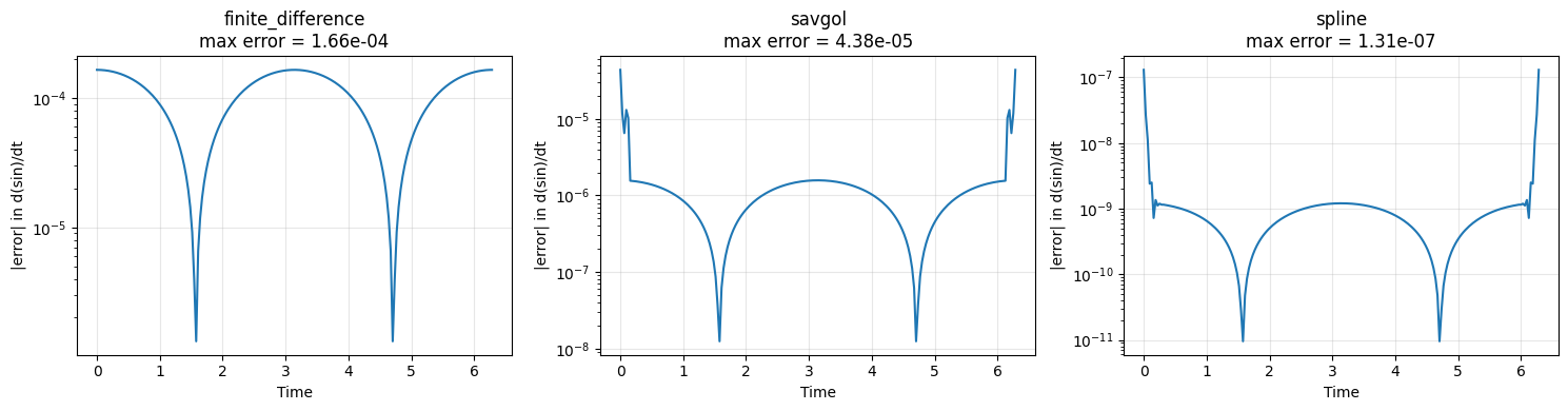
The quality of derivative estimates directly affects ODE discovery. JAXSR provides three methods:

Method	Pros	Cons
finite_difference	Works with non-uniform spacing	Lower accuracy, amplifies noise
savgol	Good noise smoothing	Requires uniform spacing
spline	High accuracy on smooth data	Can overfit noisy data

Let’s compare them on sinusoidal data where we know the exact derivatives.

t_sin = np.linspace(0, 2 * np.pi, 200)
X_sin = np.column_stack([np.sin(t_sin), np.cos(t_sin)])
dXdt_exact = np.column_stack([np.cos(t_sin), -np.sin(t_sin)])

methods = {
    "finite_difference": {},
    "savgol": {"window_length": 11, "polyorder": 3},
    "spline": {"smooth": 0.0},
}

fig, axes = plt.subplots(1, 3, figsize=(15, 4))

for ax, (method, kwargs) in zip(axes, methods.items(), strict=False):
    dXdt = estimate_derivatives(X_sin, t_sin, method=method, **kwargs)
    error = np.abs(dXdt[:, 0] - dXdt_exact[:, 0])
    ax.semilogy(t_sin, error, linewidth=1.5)
    ax.set_title(f"{method}\nmax error = {error.max():.2e}")
    ax.set_xlabel("Time")
    ax.set_ylabel("|error| in d(sin)/dt")
    ax.grid(True, alpha=0.3)

plt.tight_layout()
plt.show()

3. Lotka-Volterra Predator-Prey Equations

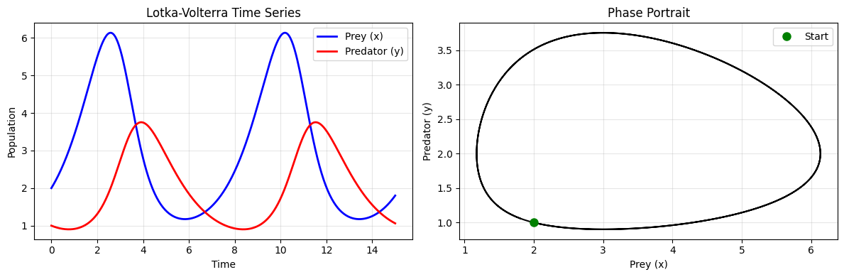
A classic coupled nonlinear ODE system:

\[\frac{dx}{dt} = \alpha\,x - \beta\,x\,y\]

\[\frac{dy}{dt} = -\gamma\,y + \delta\,x\,y\]

With parameters \(\alpha = 1.0\), \(\beta = 0.5\), \(\gamma = 0.75\), \(\delta = 0.25\).

def lotka_volterra(t, z):
    x, y = z
    return [1.0 * x - 0.5 * x * y, -0.75 * y + 0.25 * x * y]


sol = solve_ivp(
    lotka_volterra, [0, 15], [2.0, 1.0],
    t_eval=np.linspace(0, 15, 500), rtol=1e-10,
)
t_lv = sol.t
X_lv = sol.y.T  # shape (500, 2)

fig, axes = plt.subplots(1, 2, figsize=(12, 4))

axes[0].plot(t_lv, X_lv[:, 0], "b-", label="Prey (x)", linewidth=2)
axes[0].plot(t_lv, X_lv[:, 1], "r-", label="Predator (y)", linewidth=2)
axes[0].set_xlabel("Time")
axes[0].set_ylabel("Population")
axes[0].set_title("Lotka-Volterra Time Series")
axes[0].legend()
axes[0].grid(True, alpha=0.3)

axes[1].plot(X_lv[:, 0], X_lv[:, 1], "k-", linewidth=1.5)
axes[1].plot(X_lv[0, 0], X_lv[0, 1], "go", markersize=8, label="Start")
axes[1].set_xlabel("Prey (x)")
axes[1].set_ylabel("Predator (y)")
axes[1].set_title("Phase Portrait")
axes[1].legend()
axes[1].grid(True, alpha=0.3)

plt.tight_layout()
plt.show()

result_lv = discover_dynamics(
    X_lv,
    t_lv,
    state_names=["x", "y"],
    max_terms=5,
    strategy="greedy_forward",
    information_criterion="bic",
)

print(result_lv.summary())
print()
print("True equations:")
print("  d(x)/dt =  1.00*x - 0.50*x*y")
print("  d(y)/dt = -0.75*y + 0.25*x*y")

Discovered ODEs
========================================
d(x)/dt = y = 1.5963e-05*y^3 + 0.00175 - 0.000994*y - 0.4997*x*y + 0.9994*x
  R² = 1.0000, MSE = 5.18e-07, AIC = -5807.5, BIC = -5786.4
d(y)/dt = y = - 2.2235e-06*x^3 - 0.0009542 + 0.000358*x + 0.2498*x*y - 0.7495*y
  R² = 1.0000, MSE = 1.04e-07, AIC = -6610.8, BIC = -6589.8

True equations:
  d(x)/dt =  1.00*x - 0.50*x*y
  d(y)/dt = -0.75*y + 0.25*x*y

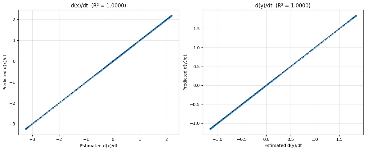
Note on spurious terms: The discovered Lotka-Volterra equations each contain 5 terms instead of the true 2 per equation. Examining the coefficients:

• For d(x)/dt: The dominant terms 0.9994*x and -0.4997*x*y recover the true coefficients (\(\alpha = 1.0\), \(\beta = 0.5\)) to within 0.1%. The three spurious terms (y^3, constant, y) all have |coefficient| < 0.002.

• For d(y)/dt: The dominant terms -0.7495*y and 0.2498*x*y recover the true coefficients (\(\gamma = 0.75\), \(\delta = 0.25\)) to within 0.2%. The spurious terms (x^3, constant, x) all have |coefficient| < 0.001.

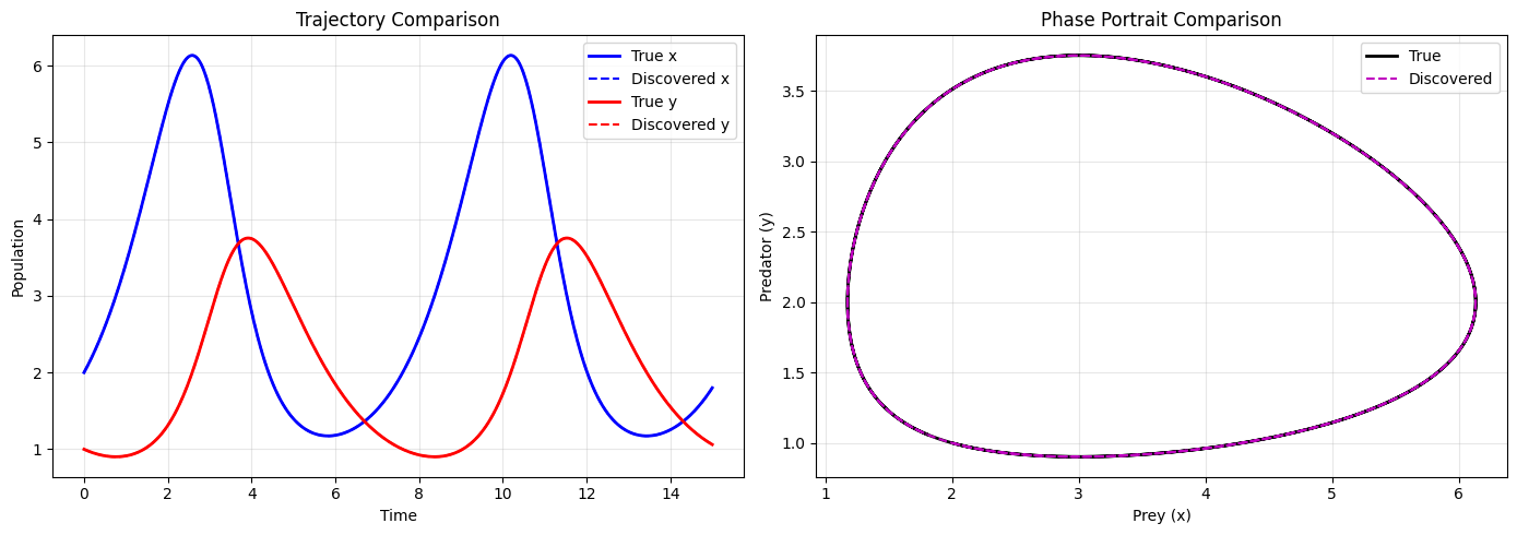
This is the same over-selection pattern seen in the exponential decay example. Greedy forward selection with BIC adds terms as long as they improve the information criterion, even when the improvement comes from fitting numerical artifacts in the derivative estimates rather than true dynamics. The spurious coefficients are negligible relative to the dominant terms and do not meaningfully affect trajectory predictions (as confirmed by the simulation in Section 6 below).

In practice, a user should inspect coefficient magnitudes relative to the dominant terms and discard any with ratios below \(\sim 10^{-3}\). Domain knowledge also helps: for Lotka-Volterra, the physics dictates that growth depends on the species’ own population and interaction terms, not on cubic terms or bare constants.

fig, axes = plt.subplots(1, 2, figsize=(12, 5))

for i, (name, ax) in enumerate(zip(["x", "y"], axes, strict=True)):
    model_i = result_lv.models[name]
    dxdt_est = result_lv.derivatives[:, i]
    dxdt_pred = np.asarray(model_i.predict(X_lv))

    ax.scatter(dxdt_est, dxdt_pred, alpha=0.3, s=10)
    lims = [min(dxdt_est.min(), dxdt_pred.min()), max(dxdt_est.max(), dxdt_pred.max())]
    ax.plot(lims, lims, "k--", linewidth=1)
    r2 = result_lv.metrics[name]["r2"]
    ax.set_xlabel(f"Estimated d({name})/dt")
    ax.set_ylabel(f"Predicted d({name})/dt")
    ax.set_title(f"d({name})/dt  (R\u00b2 = {r2:.4f})")
    ax.grid(True, alpha=0.3)

plt.tight_layout()
plt.show()

4. Noisy Data: Damped Harmonic Oscillator

Real data is noisy. Let’s test ODE discovery on a damped oscillator with added measurement noise.

The true system (written as two first-order ODEs):

\[\frac{dx_1}{dt} = x_2, \qquad \frac{dx_2}{dt} = -0.5\,x_2 - 2.0\,x_1\]

def damped_oscillator(t, z):
    x1, x2 = z
    return [x2, -0.5 * x2 - 2.0 * x1]


sol_osc = solve_ivp(
    damped_oscillator, [0, 20], [2.0, 0.0],
    t_eval=np.linspace(0, 20, 800), rtol=1e-10,
)
t_osc = sol_osc.t
X_osc_clean = sol_osc.y.T

# Add measurement noise
rng = np.random.default_rng(42)
noise_level = 0.05
X_osc = X_osc_clean + noise_level * rng.standard_normal(X_osc_clean.shape)

fig, ax = plt.subplots(figsize=(10, 4))
ax.plot(t_osc, X_osc_clean[:, 0], "b-", label="x1 (clean)", linewidth=2, alpha=0.5)
ax.plot(t_osc, X_osc[:, 0], "b.", markersize=1, label="x1 (noisy)", alpha=0.5)
ax.plot(t_osc, X_osc_clean[:, 1], "r-", label="x2 (clean)", linewidth=2, alpha=0.5)
ax.plot(t_osc, X_osc[:, 1], "r.", markersize=1, label="x2 (noisy)", alpha=0.5)
ax.set_xlabel("Time")
ax.set_ylabel("State")
ax.set_title(f"Damped Oscillator with Noise (\u03c3 = {noise_level})")
ax.legend()
ax.grid(True, alpha=0.3)
plt.tight_layout()
plt.show()

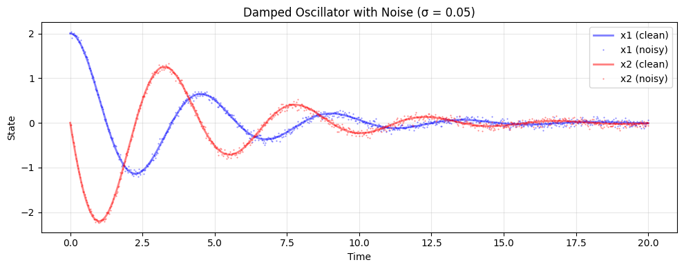
With noisy data, the Savitzky-Golay filter is a better choice for derivative estimation because it smooths the noise before differentiating.

result_osc = discover_dynamics(
    X_osc,
    t_osc,
    state_names=["x1", "x2"],
    max_terms=4,
    strategy="greedy_forward",
    information_criterion="bic",
    derivative_method="savgol",
    derivative_kw={"window_length": 15, "polyorder": 3},
)

print(result_osc.summary())
print()
print("True equations:")
print("  d(x1)/dt =  1.0*x2")
print("  d(x2)/dt = -0.5*x2 - 2.0*x1")

Discovered ODEs
========================================
d(x1)/dt = y = 0.9994*x2
  R² = 0.7851, MSE = 1.07e-01, AIC = 486.8, BIC = 491.5
d(x2)/dt = y = - 1.943*x1 - 0.4752*x2
  R² = 0.8898, MSE = 9.68e-02, AIC = 406.1, BIC = 415.5

True equations:
  d(x1)/dt =  1.0*x2
  d(x2)/dt = -0.5*x2 - 2.0*x1

5. Custom Basis Library

By default, discover_dynamics builds a library with constant, polynomial (up to degree 3), and pairwise interaction terms. You can pass a custom BasisLibrary if you have domain knowledge about the expected form of the equations.

For example, for a cubic oscillator (Duffing equation):

\[\frac{dx_1}{dt} = x_2, \qquad \frac{dx_2}{dt} = -\delta\,x_2 - \alpha\,x_1 - \beta\,x_1^3\]

alpha, beta, delta = 1.0, 0.2, 0.3


def duffing(t, z):
    x1, x2 = z
    return [x2, -delta * x2 - alpha * x1 - beta * x1**3]


sol_duf = solve_ivp(
    duffing, [0, 30], [1.5, 0.0],
    t_eval=np.linspace(0, 30, 1000), rtol=1e-10,
)
t_duf = sol_duf.t
X_duf = sol_duf.y.T

# Custom library: only include the terms we expect might appear
lib_duf = (
    BasisLibrary(n_features=2, feature_names=["x1", "x2"])
    .add_constant()
    .add_linear()                     # x1, x2
    .add_polynomials(max_degree=3)    # x1^2, x1^3, x2^2, x2^3
    .add_interactions(max_order=2)    # x1*x2
)
print(f"Custom library has {len(lib_duf)} candidate functions")

result_duf = discover_dynamics(
    X_duf,
    t_duf,
    state_names=["x1", "x2"],
    basis_library=lib_duf,
    max_terms=5,
    strategy="greedy_forward",
    information_criterion="bic",
)

print()
print(result_duf.summary())
print()
print("True equations:")
print(f"  d(x1)/dt = x2")
print(f"  d(x2)/dt = -{delta}*x2 - {alpha}*x1 - {beta}*x1^3")

Custom library has 8 candidate functions

Discovered ODEs
========================================
d(x1)/dt = y = 0.9997*x2 - 0.0005392*x1^3 - 0.0009068*x1*x2 - 0.000471*x1^2
  R² = 1.0000, MSE = 9.72e-07, AIC = -10997.9, BIC = -10978.2
d(x2)/dt = y = - x1 - 0.2998*x2 - 0.1996*x1^3 + 0.0003738*x1*x2 + 0.0001202*x1^2
  R² = 1.0000, MSE = 8.83e-08, AIC = -13394.4, BIC = -13369.8

True equations:
  d(x1)/dt = x2
  d(x2)/dt = -0.3*x2 - 1.0*x1 - 0.2*x1^3

Note on spurious terms: The discovered Duffing equations again exhibit over-selection:

• For d(x1)/dt: The dominant term 0.9997*x2 correctly recovers the true dynamics (coefficient within 0.03% of 1.0). The three spurious terms (x1^3, x1*x2, x1^2) all have |coefficient| < 0.001.

• For d(x2)/dt: The three true terms are recovered accurately: -1.000*x1 (true: -1.0), -0.2998*x2 (true: -0.3), -0.1996*x1^3 (true: -0.2). The two spurious terms (x1*x2, x1^2) have |coefficient| < 0.0004.

Recurring pattern across all examples: Greedy forward selection with BIC tends to retain a small number of spurious terms whose coefficients are orders of magnitude smaller than the true terms. This is a known limitation of BIC-penalized forward selection on finite data – the marginal reduction in residual sum of squares from fitting numerical noise can exceed BIC’s log(n) penalty when the candidate basis functions are correlated with the true signal.

Recommendations for users:

1. Always inspect coefficient magnitudes after discovery. Terms with |coefficient| orders of magnitude below the dominant terms are likely spurious.

2. Consider post-hoc thresholding: remove terms with |coefficient| < noise_level / max_basis_value.

3. Validate by simulating the discovered ODEs forward in time (as shown in Section 6). If removing small-coefficient terms does not degrade the trajectory fit, they are spurious.

4. Use domain knowledge to assess whether discovered terms are physically meaningful.

6. Simulating the Discovered Equations

A strong validation is to integrate the discovered ODEs forward in time and compare the trajectories against the original data.

# Use the Lotka-Volterra result to simulate forward
model_x = result_lv.models["x"]
model_y = result_lv.models["y"]


def discovered_rhs(t, z):
    """Right-hand side using discovered models."""
    state = np.array(z).reshape(1, -1)
    dxdt = float(model_x.predict(state)[0])
    dydt = float(model_y.predict(state)[0])
    return [dxdt, dydt]


sol_disc = solve_ivp(
    discovered_rhs, [0, 15], [2.0, 1.0],
    t_eval=t_lv, rtol=1e-8,
)

fig, axes = plt.subplots(1, 2, figsize=(14, 5))

axes[0].plot(t_lv, X_lv[:, 0], "b-", label="True x", linewidth=2)
axes[0].plot(sol_disc.t, sol_disc.y[0], "b--", label="Discovered x", linewidth=1.5)
axes[0].plot(t_lv, X_lv[:, 1], "r-", label="True y", linewidth=2)
axes[0].plot(sol_disc.t, sol_disc.y[1], "r--", label="Discovered y", linewidth=1.5)
axes[0].set_xlabel("Time")
axes[0].set_ylabel("Population")
axes[0].set_title("Trajectory Comparison")
axes[0].legend()
axes[0].grid(True, alpha=0.3)

axes[1].plot(X_lv[:, 0], X_lv[:, 1], "k-", label="True", linewidth=2)
axes[1].plot(sol_disc.y[0], sol_disc.y[1], "m--", label="Discovered", linewidth=1.5)
axes[1].set_xlabel("Prey (x)")
axes[1].set_ylabel("Predator (y)")
axes[1].set_title("Phase Portrait Comparison")
axes[1].legend()
axes[1].grid(True, alpha=0.3)

plt.tight_layout()
plt.show()

Summary

Function	Purpose
estimate_derivatives(X, t, method)	Compute dX/dt from time-series data
discover_dynamics(X, t, ...)	End-to-end ODE discovery
DynamicsResult.summary()	Human-readable output

Tips for best results:

• Use derivative_method="savgol" for noisy data

• Use derivative_method="spline" for clean, smooth data

• Pass a custom basis_library if you have domain knowledge about expected terms

• Validate by simulating the discovered ODEs forward in time

• For highly stiff or chaotic systems, use more data points and a smaller time interval

References

The SINDy approach used in this notebook builds on a rich literature connecting sparse regression, neural networks, and dynamical systems discovery:

1. Brunton, S. L., Proctor, J. L., & Kutz, J. N. (2016). Discovering governing equations from data by sparse identification of nonlinear dynamical systems. PNAS, 113(15), 3932-3937. doi:10.1073/pnas.1517384113 — The original SINDy paper that introduced sparse regression for ODE discovery.

2. Chen, R. T. Q., Rubanova, Y., Bettencourt, J., & Duvenaud, D. (2018). Neural Ordinary Differential Equations. NeurIPS 2018 (Best Paper Award). arXiv:1806.07366 — Parameterizes dynamics with neural networks and solves with ODE integrators; an alternative to SINDy that trades interpretability for flexibility.

3. Cranmer, M., Sanchez Gonzalez, A., Battaglia, P., et al. (2020). Discovering Symbolic Models from Deep Learning with Inductive Biases. NeurIPS 2020. arXiv:2006.11287 — Distills interpretable symbolic expressions from graph neural networks, bridging neural ODEs and symbolic regression.

4. Cranmer, M. (2023). Interpretable Machine Learning for Science with PySR and SymbolicRegression.jl. arXiv:2305.01582 — High-performance symbolic regression via evolutionary search; a complementary approach to the sparse-regression method used here.

5. Lemos, P., Jeffrey, N., Cranmer, M., Ho, S., & Battaglia, P. (2023). Rediscovering orbital mechanics with machine learning. Machine Learning: Science and Technology, 4(4), 045002. arXiv:2202.02306 — Recovers Newton’s law of gravitation from solar system trajectory data using graph neural networks and symbolic regression.

6. Nayek, R., Worden, K., & Cross, E. J. (2025). An Empirical Investigation of Neural ODEs and Symbolic Regression for Dynamical Systems. arXiv:2601.20637 — Compares neural ODEs and symbolic regression for discovering governing equations, showing that NODEs can augment data for symbolic regression on noisy systems.