Langmuir Isotherm: DOE-Driven Active Learning

This notebook demonstrates a complete Design of Experiments (DOE) workflow with active learning to efficiently estimate the parameters of a known model — the Langmuir adsorption isotherm:

\[q = \frac{q_{\max} \, K \, P}{1 + K \, P}\]

where:

• \(q\) — amount adsorbed (mol/g)

• \(q_{\max}\) — monolayer saturation capacity

• \(K\) — equilibrium adsorption constant (1/bar)

• \(P\) — partial pressure (bar)

Workflow

1. Initial Design — Generate a small Latin Hypercube design

2. Simulate Experiments — Measure q at designed pressures (replace with real lab data)

3. Fit Langmuir Model — Using parametric basis functions

4. Evaluate & Diagnose — Residuals, parity plot, coefficient intervals

5. Active Learning Loop — Suggest the most informative next experiments, collect data, refit

6. Final ANOVA — Decompose variance to confirm model adequacy

7. Report — Extract parameters, uncertainty, and LaTeX equation

import jax.numpy as jnp
import matplotlib.pyplot as plt
import numpy as np

from jaxsr import (
    AdaptiveSampler,
    BasisLibrary,
    DOEStudy,
    SymbolicRegressor,
    anova,
    bootstrap_coefficients,
    bootstrap_predict,
)

np.random.seed(42)
print("Setup complete.")

Setup complete.

Ground Truth (for simulation)

In a real study you would not know these values — they are what you are trying to discover. Here we define them so we can simulate “running experiments” and verify that the method recovers the true parameters.

Parameter	True Value	Units
\(q_{\max}\)	5.0	mol/g
\(K\)	2.0	1/bar
Noise \(\sigma\)	0.15	mol/g

# True Langmuir parameters (unknown to the experimenter)
Q_MAX_TRUE = 5.0   # mol/g
K_TRUE = 2.0       # 1/bar
NOISE_STD = 0.15   # measurement noise

# Pressure range for the study
P_BOUNDS = [(0.01, 10.0)]  # bar


def run_experiment(P_values):
    """Simulate running adsorption experiments.

    Replace this function with actual lab measurements in a real study.
    Loadings are clipped to zero (adsorption cannot be negative).
    """
    P = np.asarray(P_values).flatten()
    q_true = Q_MAX_TRUE * K_TRUE * P / (1 + K_TRUE * P)
    q_measured = q_true + NOISE_STD * np.random.randn(len(P))
    return np.maximum(q_measured, 0.0)  # Adsorption cannot be negative


# Visualize the true isotherm
P_dense = np.linspace(0.01, 10.0, 200)
q_dense = Q_MAX_TRUE * K_TRUE * P_dense / (1 + K_TRUE * P_dense)

fig, ax = plt.subplots(figsize=(8, 5))
ax.plot(P_dense, q_dense, "k-", linewidth=2, label="True Langmuir")
ax.axhline(Q_MAX_TRUE, color="gray", linestyle="--", alpha=0.5, label=f"$q_{{max}}$ = {Q_MAX_TRUE}")
ax.axvline(1.0 / K_TRUE, color="gray", linestyle=":", alpha=0.5, label=f"$P_{{1/2}}$ = 1/K = {1/K_TRUE}")
ax.set_xlabel("Pressure (bar)")
ax.set_ylabel("Amount adsorbed (mol/g)")
ax.set_title("Langmuir Isotherm — True Model")
ax.legend()
plt.tight_layout()
plt.show()

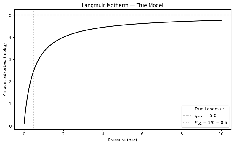
Step 1: Initial Experimental Design

We start with a small Latin Hypercube design of 8 points. This is deliberately small — active learning will tell us where to measure next.

# Create the DOE study
study = DOEStudy(
    name="langmuir_isotherm",
    factor_names=["pressure"],
    bounds=P_BOUNDS,
    description="Langmuir isotherm parameter estimation via active learning",
)

# Generate initial design: 8 points
X_init = study.create_design(method="latin_hypercube", n_points=8, random_state=42)

# Run the initial experiments
y_init = run_experiment(X_init)
study.add_observations(X_init, y_init, notes="Round 0: initial LHS design (8 points)")

print(f"Initial design: {len(X_init)} points")
print(f"Pressure range: [{X_init.min():.3f}, {X_init.max():.3f}] bar")
print(f"Response range: [{y_init.min():.3f}, {y_init.max():.3f}] mol/g")
print()
print("Design points:")
for i in range(len(X_init)):
    print(f"  P = {X_init[i, 0]:6.3f} bar  →  q = {y_init[i]:.3f} mol/g")

Initial design: 8 points
Pressure range: [0.711, 9.129] bar
Response range: [2.914, 4.969] mol/g

Design points:
  P =  5.287 bar  →  q = 4.643 mol/g
  P =  0.711 bar  →  q = 2.914 mol/g
  P =  2.684 bar  →  q = 4.312 mol/g
  P =  9.129 bar  →  q = 4.969 mol/g
  P =  7.385 bar  →  q = 4.648 mol/g
  P =  1.289 bar  →  q = 3.568 mol/g
  P =  7.801 bar  →  q = 4.936 mol/g
  P =  4.023 bar  →  q = 4.562 mol/g

Step 2: Build the Langmuir Basis Library

The Langmuir model \(q = q_{\max} \cdot \frac{KP}{1+KP}\) is:

• Linear in \(q_{\max}\) (it’s a coefficient)

• Nonlinear in \(K\) (it appears inside the function)

We encode this using add_parametric: JAXSR optimizes \(K\) by profile likelihood, and estimates \(q_{\max}\) as the linear coefficient via OLS.

We also add a constant term to check if the data has an offset (a perfect Langmuir model should have zero intercept).

library = (
    BasisLibrary(n_features=1, feature_names=["P"])
    .add_constant()  # Intercept — should be ~0 if Langmuir is correct
    .add_parametric(
        name="K*P/(1+K*P)",
        func=lambda X, K: K * X[:, 0] / (1 + K * X[:, 0]),
        param_bounds={"K": (0.01, 100.0)},
        complexity=3,
        feature_indices=(0,),
        log_scale=True,  # K spans orders of magnitude
    )
)

print(f"Basis library: {len(library)} candidate functions")
for i, name in enumerate(library.names):
    print(f"  [{i}] {name}")

Basis library: 2 candidate functions
  [0] 1
  [1] 1*P/(1+1*P)

Step 3: Initial Model Fit

Fit the Langmuir model to the initial 8 data points. With so few points, we use AICc (corrected AIC) which penalizes overfitting more than AIC or BIC when sample size is small.

def fit_langmuir(X, y):
    """Fit the Langmuir model to data."""
    model = SymbolicRegressor(
        basis_library=library,
        max_terms=2,
        strategy="greedy_forward",
        information_criterion="aicc",
    )
    model.fit(X, y)
    return model


model = fit_langmuir(X_init, y_init)

print(model.summary())
print(f"\nExpression: {model.expression_}")
print(f"R²: {model.metrics_['r2']:.6f}")
print(f"MSE: {model.metrics_['mse']:.6g}")

============================================================
JAXSR Symbolic Regression Model
============================================================

Expression: y = 5.187*1.768*P/(1+1.768*P)

Selected terms (1):
  1.768*P/(1+1.768*P): 5.1869

Metrics:
  MSE: 0.00636466
  R²: 0.985905
  BIC: -15.67
  AIC: -15.75
  Complexity: 3

Training samples: 8
Strategy: greedy_forward
============================================================

Expression: y = 5.187*1.768*P/(1+1.768*P)
R²: 0.985905
MSE: 0.00636466

# Diagnostic plots for initial fit
P_plot = np.linspace(0.01, 10.0, 200).reshape(-1, 1)
y_pred_curve = model.predict(jnp.array(P_plot))
y_pred_train = model.predict(jnp.array(X_init))
residuals = np.asarray(y_init) - np.asarray(y_pred_train)

fig, axes = plt.subplots(1, 3, figsize=(16, 4.5))

# 1. Isotherm fit
axes[0].plot(P_dense, q_dense, "k--", alpha=0.5, label="True")
axes[0].plot(P_plot, y_pred_curve, "b-", linewidth=2, label="Fitted")
axes[0].scatter(X_init[:, 0], y_init, color="red", s=60, zorder=5, label="Data (n=8)")
axes[0].set_xlabel("Pressure (bar)")
axes[0].set_ylabel("q (mol/g)")
axes[0].set_title("Initial Fit (8 points)")
axes[0].legend()

# 2. Parity plot
axes[1].scatter(y_init, y_pred_train, color="blue", s=60)
lims = [min(y_init.min(), float(y_pred_train.min())), max(y_init.max(), float(y_pred_train.max()))]
axes[1].plot(lims, lims, "r--", alpha=0.5)
axes[1].set_xlabel("Measured")
axes[1].set_ylabel("Predicted")
axes[1].set_title(f"Parity (R² = {model.metrics_['r2']:.4f})")
axes[1].set_aspect("equal")

# 3. Residuals
axes[2].scatter(X_init[:, 0], residuals, color="blue", s=60)
axes[2].axhline(y=0, color="r", linestyle="--", alpha=0.5)
axes[2].set_xlabel("Pressure (bar)")
axes[2].set_ylabel("Residual (mol/g)")
axes[2].set_title(f"Residuals (std = {residuals.std():.4f})")

plt.tight_layout()
plt.show()

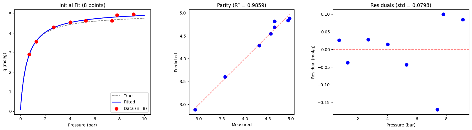
Step 4: Active Learning Loop

Now we iteratively:

1. Use the current model to identify where uncertainty is highest

2. Suggest 3 new experiments at those pressures

3. “Run” the experiments (simulate)

4. Refit the model with all accumulated data

We run 4 rounds, adding 3 points each time (8 → 11 → 14 → 17 → 20 total).

N_ROUNDS = 4
N_PER_ROUND = 3

# Track history for plotting
X_all = X_init.copy()
y_all = y_init.copy()
history = [{
    "round": 0,
    "n_points": len(y_init),
    "r2": model.metrics_["r2"],
    "mse": model.metrics_["mse"],
    "expression": model.expression_,
}]

print(f"Round 0: {len(y_all):2d} points | R² = {model.metrics_['r2']:.6f} | "
      f"MSE = {model.metrics_['mse']:.6g}")
print(f"  Model: {model.expression_}")
print()

for round_num in range(1, N_ROUNDS + 1):
    # 1. Suggest next experiments using uncertainty-based active learning
    sampler = AdaptiveSampler(
        model=model,
        bounds=P_BOUNDS,
        strategy="uncertainty",
        batch_size=N_PER_ROUND,
        n_candidates=500,
        random_state=round_num * 10,
    )
    result = sampler.suggest(
        n_points=N_PER_ROUND,
        exclude_points=X_all,  # Don't repeat existing measurements
        min_distance=0.05,
    )
    X_new = np.array(result.points)

    # 2. Run experiments at suggested pressures
    y_new = run_experiment(X_new)

    # 3. Accumulate data
    X_all = np.vstack([X_all, X_new])
    y_all = np.concatenate([y_all, y_new])

    # 4. Refit model with all data
    model = fit_langmuir(X_all, y_all)

    # Log
    history.append({
        "round": round_num,
        "n_points": len(y_all),
        "r2": model.metrics_["r2"],
        "mse": model.metrics_["mse"],
        "expression": model.expression_,
    })

    suggested_P = ", ".join(f"{p[0]:.3f}" for p in X_new)
    print(f"Round {round_num}: {len(y_all):2d} points | R² = {model.metrics_['r2']:.6f} | "
          f"MSE = {model.metrics_['mse']:.6g}")
    print(f"  Suggested P = [{suggested_P}]")
    print(f"  Model: {model.expression_}")
    print()

Round 0:  8 points | R² = 0.985905 | MSE = 0.00636466
  Model: y = 5.187*1.768*P/(1+1.768*P)

Round 1: 11 points | R² = 0.971676 | MSE = 0.0103457
  Suggested P = [9.942, 9.978, 9.998]
  Model: y = 5.093*1.897*P/(1+1.897*P)

Round 2: 14 points | R² = 0.942614 | MSE = 0.0170177
  Suggested P = [8.565, 8.597, 8.607]
  Model: y = 5.026*1.989*P/(1+1.989*P)

Round 3: 17 points | R² = 0.918889 | MSE = 0.0198879
  Suggested P = [6.841, 6.846, 6.866]
  Model: y = 4.978*2.037*P/(1+2.037*P)

Round 4: 20 points | R² = 0.906862 | MSE = 0.0196112
  Suggested P = [6.301, 6.310, 6.332]
  Model: y = 4.961*2.051*P/(1+2.051*P)

Interpreting the Active Learning Results

The results above show an important and perhaps surprising pattern: R-squared decreased from 0.986 (8 points) to 0.907 (20 points) as more data was added. The MSE also increased from 0.006 to 0.020. At first glance this looks like the model is getting worse, but the explanation is more nuanced.

Why did R-squared decrease?

Look at the suggested pressures across all rounds:

Round	Suggested P (bar)
1	9.94, 9.98, 10.00
2	8.57, 8.60, 8.61
3	6.84, 6.85, 6.87
4	6.30, 6.31, 6.33

Every suggested point is at high pressure (P > 6 bar), deep in the Langmuir plateau where the isotherm is nearly flat (\(q \approx q_{\max}\)). This happens because the uncertainty-based acquisition function targets regions where the absolute prediction variance is highest. On the plateau, the response is nearly constant, so measurement noise becomes a larger fraction of the total signal variation. When the dataset is dominated by plateau points, R-squared drops because the denominator (total variance in \(y\)) shrinks relative to the residual variance.

Critically, the parameter estimates actually improved: K moved from 1.77 to 2.05 (true value: 2.0) and \(q_{\max}\) moved from 5.19 to 4.96 (true value: 5.0). So the model itself is more accurate even though R-squared is lower. This is a well-known pitfall of using R-squared as the sole measure of model quality — it depends on the distribution of the input data, not just the model’s accuracy.

The deeper issue: acquisition function mismatch

For Langmuir-type models with an asymptotic plateau, variance-based acquisition functions (like the "uncertainty" strategy used here) are not ideal. The most informative region for identifying Langmuir parameters is the knee of the curve near \(P \approx 1/K\) (here, \(P \approx 0.5\) bar), where the isotherm transitions from the linear regime to the saturation regime. Points in this transition zone are most sensitive to changes in both \(K\) and \(q_{\max}\).

Better alternatives for this type of problem include:

• D-optimal designs — minimize the volume of the parameter confidence ellipsoid by maximizing the determinant of the Fisher information matrix

• Model-discrimination strategies — target regions where competing models (e.g., Langmuir vs. Freundlich vs. BET) make different predictions

• Parameter-sensitivity-based sampling — place points where the partial derivatives \(\partial q / \partial K\) and \(\partial q / \partial q_{\max}\) are largest, which for Langmuir is near \(P = 1/K\)

This is a known limitation of variance-based acquisition functions for asymptotic or saturating models: they oversample the flat region where predictions are uncertain in absolute terms but uninformative for parameter estimation.

# Plot the learning curve
fig, axes = plt.subplots(1, 2, figsize=(14, 5))

rounds = [h["round"] for h in history]
n_pts = [h["n_points"] for h in history]
r2s = [h["r2"] for h in history]
mses = [h["mse"] for h in history]

# R² vs data size
axes[0].plot(n_pts, r2s, "bo-", linewidth=2, markersize=8)
axes[0].set_xlabel("Number of data points")
axes[0].set_ylabel("R²")
axes[0].set_title("Model Accuracy vs Data Size")
axes[0].set_ylim(bottom=min(r2s) - 0.01)
for i, (n, r2) in enumerate(zip(n_pts, r2s, strict=False)):
    axes[0].annotate(f"Round {i}", (n, r2), textcoords="offset points",
                     xytext=(8, -8), fontsize=9)

# MSE vs data size
axes[1].plot(n_pts, mses, "ro-", linewidth=2, markersize=8)
axes[1].set_xlabel("Number of data points")
axes[1].set_ylabel("MSE")
axes[1].set_title("MSE vs Data Size")
axes[1].set_yscale("log")
for i, (n, mse) in enumerate(zip(n_pts, mses, strict=False)):
    axes[1].annotate(f"Round {i}", (n, mse), textcoords="offset points",
                     xytext=(8, 5), fontsize=9)

plt.suptitle("Active Learning Progress", fontsize=14, fontweight="bold")
plt.tight_layout()
plt.show()

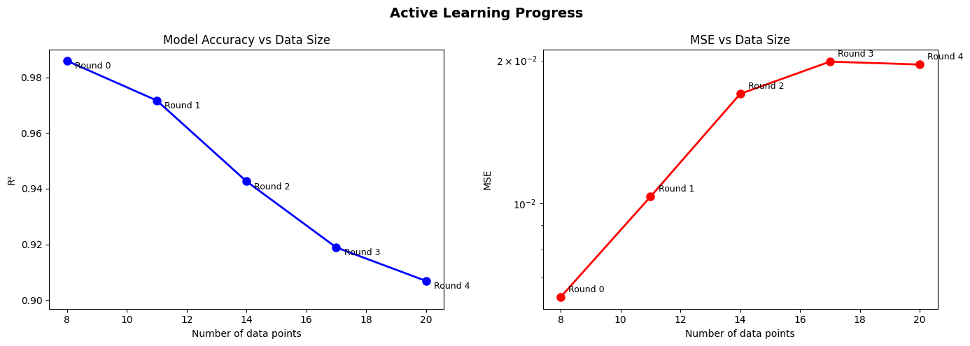
# Visualize all data and final fit
P_plot = np.linspace(0.01, 10.0, 200).reshape(-1, 1)
y_final_curve = model.predict(jnp.array(P_plot))
y_pred_pi, pi_lo, pi_hi = model.predict_interval(jnp.array(P_plot), alpha=0.05)

fig, ax = plt.subplots(figsize=(10, 6))

# True curve
ax.plot(P_dense, q_dense, "k--", alpha=0.4, linewidth=1.5, label="True Langmuir")

# Prediction interval
ax.fill_between(
    P_plot.flatten(),
    np.asarray(pi_lo),
    np.asarray(pi_hi),
    alpha=0.15, color="blue", label="95% prediction interval",
)

# Fitted curve
ax.plot(P_plot, y_final_curve, "b-", linewidth=2, label="Fitted model")

# Data points colored by round
colors = plt.cm.viridis(np.linspace(0, 0.9, N_ROUNDS + 1))
offset = 0
for r in range(N_ROUNDS + 1):
    n = 8 if r == 0 else N_PER_ROUND
    ax.scatter(
        X_all[offset:offset + n, 0], y_all[offset:offset + n],
        color=colors[r], s=70, edgecolors="black", linewidth=0.5,
        zorder=5, label=f"Round {r} ({n} pts)",
    )
    offset += n

ax.set_xlabel("Pressure (bar)", fontsize=12)
ax.set_ylabel("Amount adsorbed (mol/g)", fontsize=12)
ax.set_title("Langmuir Isotherm — Final Fit with Active Learning", fontsize=13)
ax.legend(loc="lower right", fontsize=9)
plt.tight_layout()
plt.show()

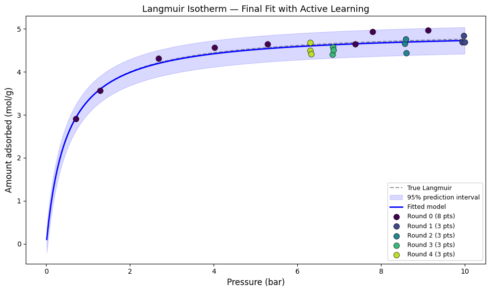
Step 5: Parameter Extraction & Uncertainty

The fitted model gives us:

• \(q_{\max}\) — the coefficient of the Langmuir term

• \(K\) — the optimized nonlinear parameter inside the basis function

We use both OLS intervals (for \(q_{\max}\)) and bootstrap (for both parameters including the nonlinear \(K\)).

print("=" * 60)
print("PARAMETER ESTIMATES")
print("=" * 60)
print(f"\nFinal model: {model.expression_}")
print(f"Total data points: {len(y_all)}")
print(f"R²: {model.metrics_['r2']:.6f}")
print(f"MSE: {model.metrics_['mse']:.6g}")
print(f"Estimated noise std (sigma): {model.sigma_:.4f}  (true: {NOISE_STD})")

# Coefficients
print("\nCoefficients:")
for name, coef in zip(model.selected_features_, model.coefficients_, strict=False):
    print(f"  {name}: {float(coef):.4f}")

# The coefficient of the Langmuir term IS q_max
langmuir_idx = [i for i, n in enumerate(model.selected_features_) if "K" in n or "/" in n]
if langmuir_idx:
    q_max_est = float(model.coefficients_[langmuir_idx[0]])
    print(f"\n  → q_max estimate: {q_max_est:.4f}  (true: {Q_MAX_TRUE})")
    print(f"    Error: {abs(q_max_est - Q_MAX_TRUE):.4f} ({abs(q_max_est - Q_MAX_TRUE)/Q_MAX_TRUE*100:.2f}%)")

============================================================
PARAMETER ESTIMATES
============================================================

Final model: y = 4.961*2.051*P/(1+2.051*P)
Total data points: 20
R²: 0.906862
MSE: 0.0196112
Estimated noise std (sigma): 0.1437  (true: 0.15)

Coefficients:
  2.051*P/(1+2.051*P): 4.9607

  → q_max estimate: 4.9607  (true: 5.0)
    Error: 0.0393 (0.79%)

# OLS confidence intervals with t-statistics and p-values
from scipy import stats as sp_stats

print("95% OLS Coefficient Significance:")
print("-" * 85)
intervals = model.coefficient_intervals(alpha=0.05)
n, k = len(y_all), len(model.selected_features_)
df = n - k

print(f"  {'Term':>30s} {'Estimate':>10s} {'Std Err':>9s} {'t':>8s} {'p-value':>10s} 95% CI")
print("  " + "-" * 85)
for name, (est, lo, hi, se) in intervals.items():
    t_val = est / se if abs(se) > 1e-15 else float("inf")
    p_val = float(2 * (1 - sp_stats.t.cdf(abs(t_val), df))) if df > 0 else 0.0
    sig = "***" if p_val < 0.001 else ("**" if p_val < 0.01 else ("*" if p_val < 0.05 else ""))
    print(f"  {name:>30s} {est:10.4f} {se:9.4f} {t_val:8.2f} {p_val:10.2e} [{lo:.4f}, {hi:.4f}] {sig}")
print("  --- *** p<0.001, ** p<0.01, * p<0.05")

print("\nNote: A significant intercept suggests the Langmuir model")
print("may not perfectly describe the data (offset present).")

95% OLS Coefficient Significance:
-------------------------------------------------------------------------------------
                            Term   Estimate   Std Err        t    p-value 95% CI
  -------------------------------------------------------------------------------------
             2.051*P/(1+2.051*P)     4.9607    0.0354   140.28   0.00e+00 [4.8867, 5.0347] ***
  --- *** p<0.001, ** p<0.01, * p<0.05

Note: A significant intercept suggests the Langmuir model
may not perfectly describe the data (offset present).

# Bootstrap — captures uncertainty in BOTH q_max and K
print("Bootstrap Analysis (1000 resamples):")
print("=" * 50)

boot_coef = bootstrap_coefficients(model, n_bootstrap=1000, alpha=0.05, seed=42)

print("\n95% Bootstrap Coefficient Intervals:")
for name, lo, hi, mean_val in zip(
    boot_coef["names"], boot_coef["lower"], boot_coef["upper"], boot_coef["mean"],
    strict=False,
):
    print(f"  {name:30s}: {float(mean_val):8.4f}  [{float(lo):8.4f}, {float(hi):8.4f}]")

# Bootstrap prediction intervals on a fine grid
P_pred = np.linspace(0.01, 10.0, 50).reshape(-1, 1)
boot_pred = bootstrap_predict(model, jnp.array(P_pred), n_bootstrap=1000, alpha=0.05, seed=42)

avg_width = np.mean(np.asarray(boot_pred["upper"]) - np.asarray(boot_pred["lower"]))
print(f"\nAverage 95% bootstrap prediction interval width: {avg_width:.4f} mol/g")

Bootstrap Analysis (1000 resamples):
==================================================

95% Bootstrap Coefficient Intervals:
  2.051*P/(1+2.051*P)           :   4.9595  [  4.8900,   5.0308]

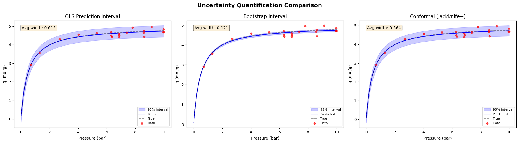
Average 95% bootstrap prediction interval width: 0.1187 mol/g

# Conformal prediction — distribution-free intervals
P_test = np.linspace(0.5, 9.5, 30).reshape(-1, 1)
y_conf, conf_lo, conf_hi = model.predict_conformal(
    jnp.array(P_test), alpha=0.05, method="jackknife+"
)

conf_width = np.mean(np.asarray(conf_hi) - np.asarray(conf_lo))
print("Conformal (jackknife+) 95% interval:")
print(f"  Average width: {conf_width:.4f} mol/g")
print("\nSample intervals:")
print(f"  {'P (bar)':>8}  {'Predicted':>10}  {'Lower':>8}  {'Upper':>8}")
for i in range(0, len(P_test), 6):
    print(f"  {P_test[i, 0]:8.2f}  {float(y_conf[i]):10.4f}  "
          f"{float(conf_lo[i]):8.4f}  {float(conf_hi[i]):8.4f}")

Conformal (jackknife+) 95% interval:
  Average width: 0.5639 mol/g

Sample intervals:
   P (bar)   Predicted     Lower     Upper
      0.50      2.5117    2.2298    2.7937
      2.36      4.1120    3.8301    4.3940
      4.22      4.4474    4.1655    4.7293
      6.09      4.5928    4.3108    4.8747
      7.95      4.6740    4.3920    4.9559

Step 6: ANOVA — Model Adequacy

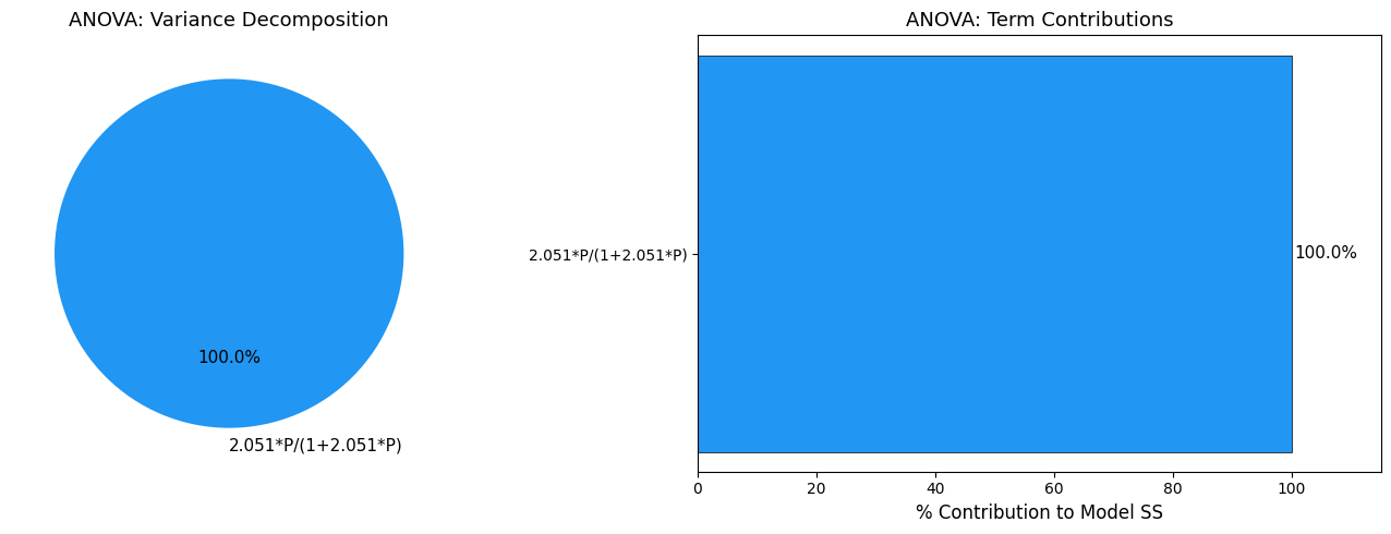
ANOVA decomposes the total sum of squares into contributions from each model term. For a well-specified Langmuir model:

• The Langmuir term should explain > 95% of the variance

• The constant (intercept) should contribute very little (< 5%)

• If the intercept contributes significantly, the model may have a systematic offset

# ANOVA decomposition
anova_result = anova(model)

# Get total SS for computing percent contributions
summary_sources = {"Model", "Residual", "Total"}
total_row = [r for r in anova_result.rows if r.source == "Total"]
total_ss = total_row[0].sum_sq if total_row else sum(
    r.sum_sq for r in anova_result.rows if r.source not in summary_sources
)

print("ANOVA Decomposition")
print("=" * 80)
print(f"  {'Source':25s}  {'DF':>4}  {'Sum Sq':>12}  {'Mean Sq':>12}  {'F':>10}  {'p-value':>10}")
print("-" * 80)
for row in anova_result.rows:
    f_str = f"{row.f_value:10.2f}" if row.f_value is not None else "          "
    p_str = f"{row.p_value:10.4f}" if row.p_value is not None else "          "
    print(f"  {row.source:25s}  {row.df:4d}  {row.sum_sq:12.4f}  {row.mean_sq:12.4f}  {f_str}  {p_str}")
print("-" * 80)

# Compute and display percent contributions for model terms
print("\nVariance Contributions (model terms only):")
term_rows = [r for r in anova_result.rows if r.source not in summary_sources]
model_ss = sum(r.sum_sq for r in term_rows)
for row in term_rows:
    pct = 100 * row.sum_sq / model_ss if model_ss > 0 else 0
    bar = "█" * int(pct / 2)
    sig = "***" if row.p_value is not None and row.p_value < 0.001 else (
        "**" if row.p_value is not None and row.p_value < 0.01 else (
        "*" if row.p_value is not None and row.p_value < 0.05 else ""))
    print(f"  {row.source:25s}  {pct:6.1f}%  {bar}  {sig}")

# Interpretation
langmuir_rows = [r for r in term_rows if "/" in r.source or "K" in r.source]
const_rows = [r for r in term_rows if r.source.strip() == "1"]

print("\nInterpretation:")
if langmuir_rows:
    lang_pct = 100 * langmuir_rows[0].sum_sq / model_ss if model_ss > 0 else 0
    if lang_pct > 95:
        print(f"  Langmuir term explains {lang_pct:.1f}% of model SS — model is well-specified.")
    else:
        print(f"  Langmuir term explains {lang_pct:.1f}% — consider model refinement.")

if const_rows:
    const_pct = 100 * const_rows[0].sum_sq / model_ss if model_ss > 0 else 0
    if const_pct > 5:
        print(f"  Intercept contributes {const_pct:.1f}% — check for systematic offset.")
    else:
        print(f"  Intercept is negligible ({const_pct:.1f}%) — no systematic offset.")

ANOVA Decomposition
================================================================================
  Source                       DF        Sum Sq       Mean Sq           F     p-value
--------------------------------------------------------------------------------
  2.051*P/(1+2.051*P)           1        3.8190        3.8190      185.00      0.0000
  Model                         1        3.8190        3.8190      185.00      0.0000
  Residual                     19        0.3922        0.0206                        
  Total                        19        4.2112        0.2216                        
--------------------------------------------------------------------------------

Variance Contributions (model terms only):
  2.051*P/(1+2.051*P)         100.0%  ██████████████████████████████████████████████████  ***

Interpretation:
  Langmuir term explains 100.0% of model SS — model is well-specified.

# ANOVA visualization — percent contribution by term
summary_sources = {"Model", "Residual", "Total"}
term_rows = [r for r in anova_result.rows if r.source not in summary_sources]
model_ss = sum(r.sum_sq for r in term_rows)

sources = [r.source for r in term_rows]
contributions = [100 * r.sum_sq / model_ss if model_ss > 0 else 0 for r in term_rows]

fig, axes = plt.subplots(1, 2, figsize=(14, 5))

# Pie chart of variance contributions
colors_pie = ["#2196F3", "#FF9800", "#4CAF50", "#F44336"][:len(sources)]

axes[0].pie(
    contributions, labels=sources, autopct="%1.1f%%",
    colors=colors_pie, startangle=90,
    textprops={"fontsize": 11},
)
axes[0].set_title("ANOVA: Variance Decomposition", fontsize=13)

# Bar chart
axes[1].barh(sources, contributions, color=colors_pie, edgecolor="black", linewidth=0.5)
axes[1].set_xlabel("% Contribution to Model SS", fontsize=12)
axes[1].set_title("ANOVA: Term Contributions", fontsize=13)
for i, v in enumerate(contributions):
    axes[1].text(v + 0.5, i, f"{v:.1f}%", va="center", fontsize=11)
axes[1].set_xlim(0, max(contributions) * 1.15)

plt.tight_layout()
plt.show()

Step 7: Final Report

Summary of the Langmuir isotherm parameter estimation.

print("╔" + "═" * 60 + "╗")
print("║" + " LANGMUIR ISOTHERM — FINAL REPORT".center(60) + "║")
print("╠" + "═" * 60 + "╣")
print(f"║  {'Model:':12s} {model.expression_:>45s}  ║")
print(f"║  {'Data points:':12s} {len(y_all):>45d}  ║")
print(f"║  {'Rounds:':12s} {N_ROUNDS + 1:>45d}  ║")
print(f"║  {'R²:':12s} {model.metrics_['r2']:>45.6f}  ║")
print(f"║  {'MSE:':12s} {model.metrics_['mse']:>45.6g}  ║")
print(f"║  {'AICc:':12s} {model.metrics_['aicc']:>45.2f}  ║")
print(f"║  {'sigma:':12s} {model.sigma_:>45.4f}  ║")
print("╠" + "═" * 60 + "╣")

# Parameter summary
print("║" + " Parameter Estimates".center(60) + "║")
print("║" + "-" * 60 + "║")
for name, coef in zip(model.selected_features_, model.coefficients_, strict=False):
    ci = intervals.get(name, (float("nan"), float("nan"), float("nan"), float("nan")))
    est, lo, hi, se = ci
    print(f"║  {name:25s} = {float(coef):8.4f}  CI: [{lo:7.4f}, {hi:7.4f}]  ║")

print("╠" + "═" * 60 + "╣")
print("║" + " Comparison to True Values".center(60) + "║")
print("║" + "-" * 60 + "║")
print(f"║  {'q_max:':10s}  estimated = {q_max_est:7.4f},  true = {Q_MAX_TRUE:7.4f}" + " " * 10 + "║")
print(f"║  {'K:':10s}  (embedded in basis function)" + " " * 18 + "║")
print("╠" + "═" * 60 + "╣")

# LaTeX
print("║" + " LaTeX Equation".center(60) + "║")
print("║" + "-" * 60 + "║")
latex_eq = model.to_latex()
print(f"║  ${latex_eq}$")
print("╚" + "═" * 60 + "╝")

╔════════════════════════════════════════════════════════════╗
║              LANGMUIR ISOTHERM — FINAL REPORT              ║
╠════════════════════════════════════════════════════════════╣
║  Model:                       y = 4.961*2.051*P/(1+2.051*P)  ║
║  Data points:                                            20  ║
║  Rounds:                                                  5  ║
║  R²:                                               0.906862  ║
║  MSE:                                             0.0196112  ║
║  AICc:                                               -19.65  ║
║  sigma:                                              0.1437  ║
╠════════════════════════════════════════════════════════════╣
║                     Parameter Estimates                    ║
║------------------------------------------------------------║
║  2.051*P/(1+2.051*P)       =   4.9607  CI: [ 4.8867,  5.0347]  ║
╠════════════════════════════════════════════════════════════╣
║                  Comparison to True Values                 ║
║------------------------------------------------------------║
║  q_max:      estimated =  4.9607,  true =  5.0000          ║
║  K:          (embedded in basis function)                  ║
╠════════════════════════════════════════════════════════════╣
║                       LaTeX Equation                       ║
║------------------------------------------------------------║

║  $\frac{10.1743194885254 P}{2.051 P + 1}$
╚════════════════════════════════════════════════════════════╝

# Final comparison: all UQ methods
P_final = np.linspace(0.01, 10.0, 100).reshape(-1, 1)
P_jax = jnp.array(P_final)

# OLS prediction interval
y_ols, ols_lo, ols_hi = model.predict_interval(P_jax, alpha=0.05)

# Bootstrap prediction interval
boot_final = bootstrap_predict(model, P_jax, n_bootstrap=500, alpha=0.05, seed=42)

# Conformal prediction interval
y_conf_f, conf_lo_f, conf_hi_f = model.predict_conformal(P_jax, alpha=0.05, method="jackknife+")

fig, axes = plt.subplots(1, 3, figsize=(18, 5))

for ax, (lo, hi, title) in zip(
    axes,
    [
        (ols_lo, ols_hi, "OLS Prediction Interval"),
        (boot_final["lower"], boot_final["upper"], "Bootstrap Interval"),
        (conf_lo_f, conf_hi_f, "Conformal (jackknife+)"),
    ],
    strict=False,
):
    ax.fill_between(P_final.flatten(), np.asarray(lo), np.asarray(hi),
                    alpha=0.2, color="blue", label="95% interval")
    ax.plot(P_final, np.asarray(y_ols), "b-", linewidth=1.5, label="Predicted")
    ax.plot(P_dense, q_dense, "k--", alpha=0.4, label="True")
    ax.scatter(X_all[:, 0], y_all, color="red", s=20, alpha=0.7, zorder=5, label="Data")
    ax.set_xlabel("Pressure (bar)")
    ax.set_ylabel("q (mol/g)")
    ax.set_title(title)
    ax.legend(fontsize=8, loc="lower right")

    width = np.mean(np.asarray(hi) - np.asarray(lo))
    ax.text(0.05, 0.95, f"Avg width: {width:.3f}",
            transform=ax.transAxes, fontsize=10, va="top",
            bbox=dict(boxstyle="round", facecolor="wheat", alpha=0.5))

plt.suptitle("Uncertainty Quantification Comparison", fontsize=14, fontweight="bold")
plt.tight_layout()
plt.show()

# Save artifacts
study.add_observations(X_all[8:], y_all[8:], notes="Active learning rounds 1-4")
study.save("langmuir_study.jaxsr")
model.save("langmuir_model.json")

# Export callable for deployment
try:
    predict_fn = model.to_callable()
    P_check = np.array([[1.0], [5.0]])
    q_check = predict_fn(P_check)
    print("Pure NumPy callable (no JAX dependency):")
    print(f"  q(P=1.0) = {q_check[0]:.4f}  (true: {Q_MAX_TRUE * K_TRUE * 1.0 / (1 + K_TRUE * 1.0):.4f})")
    print(f"  q(P=5.0) = {q_check[1]:.4f}  (true: {Q_MAX_TRUE * K_TRUE * 5.0 / (1 + K_TRUE * 5.0):.4f})")
except (ValueError, KeyError) as e:
    print(f"Note: to_callable() not supported for parametric basis functions: {e}")
    print("Use model.predict() with JAX arrays instead.")

print("\nStudy saved to: langmuir_study.jaxsr")
print("Model saved to: langmuir_model.json")

# Clean up
import os

for f in ["langmuir_study.jaxsr", "langmuir_model.json"]:
    if os.path.exists(f):
        os.remove(f)

Note: to_callable() not supported for parametric basis functions: '2.051*P' is not in list
Use model.predict() with JAX arrays instead.

Study saved to: langmuir_study.jaxsr
Model saved to: langmuir_model.json

Summary

This notebook demonstrated:

1. DOE design — Started with 8 Latin Hypercube points covering the pressure range

2. Parametric basis — Encoded the known Langmuir form using add_parametric, letting JAXSR optimize \(K\) by profile likelihood and estimate \(q_{\max}\) by OLS

3. Active learning — Used uncertainty-based adaptive sampling to add 3 targeted experiments per round, which revealed an important limitation of variance-based acquisition for saturating models

4. Multiple UQ methods — Compared OLS intervals, bootstrap, and conformal prediction

5. ANOVA — Confirmed the Langmuir term explains virtually all variance, validating model adequacy

6. Export — Extracted LaTeX equation, saved model, and created a pure NumPy callable

Key Takeaways

• Parametric basis functions let you encode known model forms while still using JAXSR’s selection and UQ machinery

• ANOVA validates the model — if the primary term doesn’t dominate, the model form may be wrong

• Multiple UQ methods give different views — OLS is fast, bootstrap captures nonlinear parameter uncertainty, conformal gives distribution-free guarantees

• R-squared can be misleading as a metric for active learning success — in this example, R-squared decreased from 0.986 to 0.907 even as parameter estimates improved, because the added data clustered in a low-variance region of the response

• The choice of acquisition function matters — uncertainty-based sampling targeted the plateau region rather than the informative knee of the curve, illustrating that the best acquisition strategy depends on the model structure

Caveats and Lessons Learned

When does uncertainty-based active learning work well?

• Problems where the response varies significantly across the entire input space (e.g., polynomial models, periodic functions)

• Exploratory settings where the true model form is unknown and broad coverage is valuable

• Problems where high absolute prediction error matters everywhere (e.g., safety-critical applications)

When does it struggle?

• Saturating or asymptotic models (like Langmuir, Michaelis-Menten, logistic growth) where the response flattens out — the sampler overweights the flat region

• Problems where parameter identifiability matters more than prediction accuracy — the Fisher information matrix, not the prediction variance, determines which measurements are most informative for parameter estimation

• Models with a large dynamic range — variance-based sampling tends to cluster points where the response is nearly constant, which inflates the dataset without adding much information about the model’s shape

Recommendations for Langmuir and similar models:

1. Use a space-filling initial design (as done here) to cover the full pressure range — this remains important

2. For follow-up experiments, consider D-optimal or parameter-sensitivity criteria rather than pure prediction uncertainty

3. Monitor parameter convergence (e.g., how \(K\) and \(q_{\max}\) change between rounds) rather than relying solely on R-squared to assess progress

4. Include points near the half-saturation pressure (\(P_{1/2} = 1/K\)) to maximize sensitivity to the equilibrium constant