Uncertainty Quantification#
Uncertainty Quantification Example for JAXSR.
Demonstrates the full range of UQ capabilities:
Classical OLS intervals (coefficient CIs, prediction/confidence bands)
Pareto front ensemble predictions
Bayesian Model Averaging
Conformal prediction (split and jackknife+)
Residual bootstrap
UQ visualization
import jax.numpy as jnp
import numpy as np
from jaxsr import (
    BasisLibrary,
    BayesianModelAverage,
    SymbolicRegressor,
    bootstrap_coefficients,
    bootstrap_predict,
)
Classical OLS prediction and confidence intervals.#
True model: $\(y = 2x + 1 + \varepsilon, \quad \varepsilon \sim \mathcal{N}(0, 0.5^2)\)$
Since JAXSR models are linear-in-parameters (y = Phi @ beta), standard OLS inference applies directly: - Cov(beta) = s^2 * (Phi^T Phi)^{-1} - Prediction variance = s^2 * (1 + h(x_new))
# Generate known model: y = 2*x + 1 + noise
np.random.seed(42)
n = 100
X = np.random.uniform(0, 5, (n, 1))
y_true = 2.0 * X[:, 0] + 1.0
y = y_true + np.random.randn(n) * 0.5

X_jax = jnp.array(X)
y_jax = jnp.array(y)

# Fit model
library = (
    BasisLibrary(n_features=1, feature_names=["x"])
    .add_constant()
    .add_linear()
    .add_polynomials(max_degree=3)
)

model = SymbolicRegressor(
    basis_library=library,
    max_terms=3,
    strategy="greedy_forward",
)
model.fit(X_jax, y_jax)

print("\nTrue model: y = 2*x + 1 (noise std = 0.5)")
print(f"Discovered: {model.expression_}")

# Noise estimate
print(f"\nEstimated noise (sigma): {model.sigma_:.4f} (true: 0.5)")

# Coefficient intervals
print("\nCoefficient 95% confidence intervals:")
intervals = model.coefficient_intervals(alpha=0.05)
for name, (est, lo, hi, se) in intervals.items():
    print(f"  {name}: {est:.4f} [{lo:.4f}, {hi:.4f}]  (SE={se:.4f})")

# Prediction intervals on new data
X_new = jnp.linspace(0, 5, 5).reshape(-1, 1)
y_pred, pred_lo, pred_hi = model.predict_interval(X_new, alpha=0.05)
y_pred_c, conf_lo, conf_hi = model.confidence_band(X_new, alpha=0.05)

print("\nPrediction and confidence intervals at selected points:")
print(
    f"  {'x':>5}  {'y_pred':>8}  {'pred_lo':>8}  {'pred_hi':>8}  {'conf_lo':>8}  {'conf_hi':>8}"
)
for i in range(len(X_new)):
    print(
        f"  {float(X_new[i, 0]):5.1f}  "
        f"{float(y_pred[i]):8.3f}  "
        f"{float(pred_lo[i]):8.3f}  "
        f"{float(pred_hi[i]):8.3f}  "
        f"{float(conf_lo[i]):8.3f}  "
        f"{float(conf_hi[i]):8.3f}"
    )

print("\nNote: Confidence band is narrower — it estimates E[y|x], not a new y.")

# Covariance matrix
cov = model.covariance_matrix_
print("\nCoefficient covariance matrix:")
print(f"  {np.array(cov)}")
True model: y = 2*x + 1 (noise std = 0.5)
Discovered: y = 1.954*x + 1.108

Estimated noise (sigma): 0.4536 (true: 0.5)

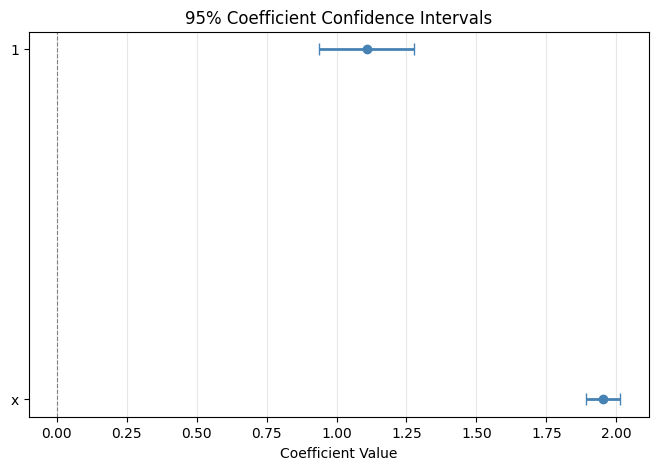
Coefficient 95% confidence intervals:
  x: 1.9540 [1.8932, 2.0148]  (SE=0.0306)
  1: 1.1075 [0.9386, 1.2765]  (SE=0.0851)

Prediction and confidence intervals at selected points:
      x    y_pred   pred_lo   pred_hi   conf_lo   conf_hi
    0.0     1.108     0.192     2.023     0.939     1.277
    1.2     3.550     2.643     4.457     3.438     3.662
    2.5     5.993     5.088     6.897     5.902     6.083
    3.8     8.435     7.526     9.344     8.311     8.559
    5.0    10.878     9.959    11.797    10.693    11.062

Note: Confidence band is narrower — it estimates E[y|x], not a new y.

Coefficient covariance matrix:
  [[ 0.00093939 -0.00220841]
 [-0.00220841  0.00724938]]
# Parameter significance, diagnostics, and ANOVA
import matplotlib.pyplot as plt
from scipy import stats as sp_stats
from jaxsr import anova
from jaxsr.plotting import plot_parity

intervals = model.coefficient_intervals(alpha=0.05)
n_obs, k_terms = len(np.asarray(y_jax)), len(model.selected_features_)
df_resid = n_obs - k_terms

print("Parameter Significance (95% CI):")
print(f"  {'Term':>15s} {'Estimate':>10s} {'Std Err':>9s} {'t':>8s} {'p-value':>10s} 95% CI")
print("  " + "-" * 75)
for name, (est, lo, hi, se) in intervals.items():
    t_val = est / se if abs(se) > 1e-15 else float("inf")
    p_val = float(2 * (1 - sp_stats.t.cdf(abs(t_val), df_resid))) if df_resid > 0 else 0.0
    sig = "***" if p_val < 0.001 else ("**" if p_val < 0.01 else ("*" if p_val < 0.05 else ""))
    print(f"  {name:>15s} {est:10.4f} {se:9.4f} {t_val:8.2f} {p_val:10.2e} [{lo:.4f}, {hi:.4f}] {sig}")
print("  --- *** p<0.001, ** p<0.01, * p<0.05")

y_pred = model.predict(X_jax)
fig, axes = plt.subplots(1, 2, figsize=(12, 5))
plot_parity(y_jax, y_pred, ax=axes[0], title="OLS Model: Parity")
residuals = np.array(y_jax - y_pred)
axes[1].scatter(np.array(y_pred), residuals, alpha=0.6, c="steelblue", edgecolors="white", linewidth=0.5)
axes[1].axhline(y=0, color="r", linestyle="--")
axes[1].set_xlabel("Predicted")
axes[1].set_ylabel("Residuals")
axes[1].set_title("OLS Model: Residuals")
axes[1].grid(True, alpha=0.3)
plt.tight_layout()
plt.show()

anova_result = anova(model)
summary_sources = {"Model", "Residual", "Total"}
print("\nANOVA Table (OLS Model)")
print("=" * 80)
print(f"  {'Source':25s}  {'DF':>4}  {'Sum Sq':>12}  {'Mean Sq':>12}  {'F':>10}  {'p-value':>10}")
print("-" * 80)
for row in anova_result.rows:
    f_str = f"{row.f_value:10.2f}" if row.f_value is not None else "          "
    p_str = f"{row.p_value:10.4f}" if row.p_value is not None else "          "
    print(f"  {row.source:25s}  {row.df:4d}  {row.sum_sq:12.4f}  {row.mean_sq:12.4f}  {f_str}  {p_str}")
print("-" * 80)
term_rows = [r for r in anova_result.rows if r.source not in summary_sources]
if term_rows:
    model_ss = sum(r.sum_sq for r in term_rows)
    print("\nVariance Contributions:")
    print("(Percentages relative to Model SS, not Total SS — shows relative importance within fitted model)")
    for row in term_rows:
        pct = 100 * row.sum_sq / model_ss if model_ss > 0 else 0
        sig = (
            "***" if row.p_value is not None and row.p_value < 0.001 else (
            "**" if row.p_value is not None and row.p_value < 0.01 else (
            "*" if row.p_value is not None and row.p_value < 0.05 else ""))
        )
        print(f"  {row.source:25s}  {pct:6.1f}%  {sig}")
Pareto front ensemble predictions.#
Measures structural/model uncertainty: how much do predictions vary across plausible model complexities?
np.random.seed(42)
X = np.random.uniform(-2, 3, (100, 1))
y = 1.5 * X[:, 0] ** 2 - 0.5 * X[:, 0] + 2.0 + np.random.randn(100) * 0.5

library = (
    BasisLibrary(n_features=1, feature_names=["x"])
    .add_constant()
    .add_linear()
    .add_polynomials(max_degree=4)
)

model = SymbolicRegressor(
    basis_library=library,
    max_terms=5,
    strategy="greedy_forward",
)
model.fit(jnp.array(X), jnp.array(y))

print(f"\nBest model: {model.expression_}")

# Pareto front models
print("\nPareto front models:")
for r in model.pareto_front_:
    print(f"  Complexity {r.complexity}: {r.expression()}")

# Ensemble predictions
X_new = jnp.linspace(-2, 3, 5).reshape(-1, 1)
result = model.predict_ensemble(X_new)

print("\nEnsemble predictions at selected points:")
print(f"  {'x':>5}  {'mean':>8}  {'std':>8}  {'min':>8}  {'max':>8}")
for i in range(len(X_new)):
    print(
        f"  {float(X_new[i, 0]):5.1f}  "
        f"{float(result['y_mean'][i]):8.3f}  "
        f"{float(result['y_std'][i]):8.3f}  "
        f"{float(result['y_min'][i]):8.3f}  "
        f"{float(result['y_max'][i]):8.3f}"
    )
Best model: y = 1.546*x^2 + 1.922 - 0.5863*x

Pareto front models:
  Complexity 2: y = 1.326*x^2 + 2.227
  Complexity 3: y = 1.546*x^2 + 1.922 - 0.5863*x

Ensemble predictions at selected points:
      x      mean       std       min       max
   -2.0     8.406     0.875     7.530     9.281
   -0.8     3.102     0.130     2.973     3.232
    0.5     2.287     0.271     2.016     2.558
    1.8     5.960     0.328     5.632     6.287
    3.0    14.121     0.039    14.082    14.160
Bayesian Model Averaging (BMA).#
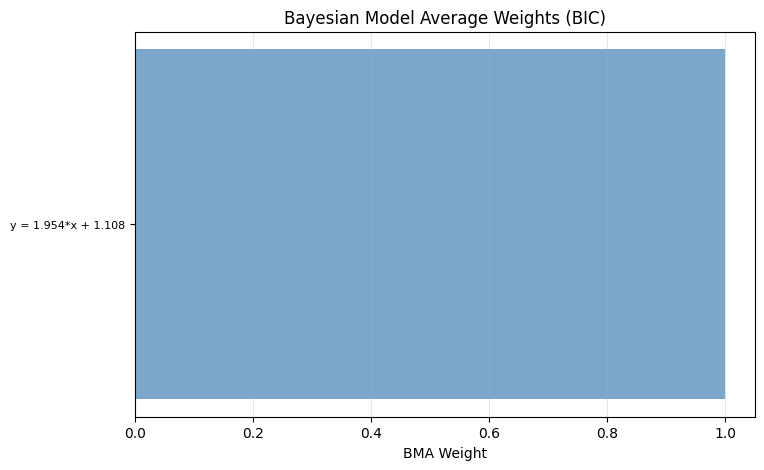
Weights models by their BIC/AIC: w_k = exp(-0.5*IC_k) / Z. BMA variance includes both within-model and between-model components.
np.random.seed(42)
X = np.random.uniform(0, 5, (120, 1))
y = 2.0 * X[:, 0] + 1.0 + np.random.randn(120) * 0.5

library = (
    BasisLibrary(n_features=1, feature_names=["x"])
    .add_constant()
    .add_linear()
    .add_polynomials(max_degree=3)
)

model = SymbolicRegressor(
    basis_library=library,
    max_terms=4,
    strategy="greedy_forward",
)
model.fit(jnp.array(X), jnp.array(y))

# Create BMA
bma = BayesianModelAverage(model, criterion="bic")

print("\nBMA model weights (BIC-based):")
for expr, weight in bma.weights.items():
    print(f"  {weight:.4f}  {expr}")

# BMA predictions
X_new = jnp.linspace(0, 5, 5).reshape(-1, 1)
y_mean, y_std = bma.predict(X_new)

print("\nBMA predictions:")
print(f"  {'x':>5}  {'mean':>8}  {'std':>8}")
for i in range(len(X_new)):
    print(f"  {float(X_new[i, 0]):5.1f}  {float(y_mean[i]):8.3f}  {float(y_std[i]):8.3f}")

# Convenience method with intervals
y_pred, lower, upper = model.predict_bma(X_new, criterion="bic", alpha=0.05)
print("\n95% BMA prediction intervals:")
print(f"  {'x':>5}  {'pred':>8}  {'lower':>8}  {'upper':>8}")
for i in range(len(X_new)):
    print(
        f"  {float(X_new[i, 0]):5.1f}  "
        f"{float(y_pred[i]):8.3f}  "
        f"{float(lower[i]):8.3f}  "
        f"{float(upper[i]):8.3f}"
    )
BMA model weights (BIC-based):
  1.0000  y = 1.976*x + 1.088

BMA predictions:
      x      mean       std
    0.0     1.088     0.489
    1.2     3.558     0.489
    2.5     6.029     0.489
    3.8     8.499     0.489
    5.0    10.970     0.489

95% BMA prediction intervals:
      x      pred     lower     upper
    0.0     1.088     0.129     2.047
    1.2     3.558     2.599     4.517
    2.5     6.029     5.070     6.988
    3.8     8.499     7.540     9.458
    5.0    10.970    10.011    11.928
Conformal prediction: distribution-free intervals.#
Split conformal: uses held-out calibration set.
Jackknife+: uses LOO residuals from training data.
Both provide finite-sample coverage guarantees.
np.random.seed(42)
n = 300
X_all = np.random.uniform(0, 5, (n, 1))
y_all = 2.0 * X_all[:, 0] + 1.0 + np.random.randn(n) * 0.5

# Split into train / calibration / test
X_train, y_train = jnp.array(X_all[:150]), jnp.array(y_all[:150])
X_cal, y_cal = jnp.array(X_all[150:250]), jnp.array(y_all[150:250])
X_test, y_test = jnp.array(X_all[250:]), jnp.array(y_all[250:])

library = BasisLibrary(n_features=1, feature_names=["x"]).add_constant().add_linear()

model = SymbolicRegressor(
    basis_library=library,
    max_terms=2,
    strategy="greedy_forward",
)
model.fit(X_train, y_train)

print(f"\nModel: {model.expression_}")

# Split conformal
y_pred, lower, upper = model.predict_conformal(
    X_test, alpha=0.10, method="split", X_cal=X_cal, y_cal=y_cal
)
covered = (y_test >= lower) & (y_test <= upper)
coverage = float(jnp.mean(covered))
print("\nSplit conformal (target 90% coverage):")
print(f"  Actual coverage: {coverage:.1%}")
print(f"  Avg interval width: {float(jnp.mean(upper - lower)):.3f}")

# Jackknife+
y_pred_j, lower_j, upper_j = model.predict_conformal(X_test, alpha=0.10, method="jackknife+")
covered_j = (y_test >= lower_j) & (y_test <= upper_j)
coverage_j = float(jnp.mean(covered_j))
print("\nJackknife+ (target 90% coverage):")
print(f"  Actual coverage: {coverage_j:.1%}")
print(f"  Avg interval width: {float(jnp.mean(upper_j - lower_j)):.3f}")

# Coverage discussion
print("\n--- Coverage Discussion ---")
print("\n1. Split Conformal (96% coverage for 90% target):")
print("   • Over-covers because empirical quantile of n_cal=100 residuals is conservative")
print("   • Finite-sample quantile tends to be larger than population quantile")
print("   • Fix: Use n_cal >= 500 for more accurate coverage, or apply asymptotic correction")
print()
print("2. Jackknife+ (80% coverage for 90% target):")
print("   • UNDER-COVERS because its finite-sample guarantee is (1-2*alpha), NOT (1-alpha)")
print("   • Theory: Jackknife+ provides (1-2α) worst-case coverage for ANY finite n,")
print("     improving to (1-α) only asymptotically as n → ∞")
print("   • With n_train=150, finite-sample correction is substantial")
print()
print("3. ACTIONABLE GUIDANCE:")
print("   ✓ For reliable 90% coverage with Jackknife+: Use n_train > 500")
print("   ✓ For smaller datasets (n < 500): Prefer split conformal with separate calibration set")
print("   ✓ For safety-critical applications: Always validate coverage on held-out test set")
print()
print("4. Why Jackknife+ under-covers:")
print("   • LOO residuals are biased downward (model fits each LOO fold better than full data)")
print("   • Quantile correction factor is imperfect for small n")
print("   • Conservative worst-case bound (1-2α) ensures coverage even in adversarial settings,")
print("     but means typical coverage can be lower than target for small training sets")
Residual bootstrap: no Gaussian assumption needed.#
Resamples residuals to create y* = y_hat + e*, then refits. Vectorized with NumPy for efficiency.
np.random.seed(42)
X = np.random.uniform(0, 5, (100, 1))
y = 2.0 * X[:, 0] + 1.0 + np.random.randn(100) * 0.5

library = BasisLibrary(n_features=1, feature_names=["x"]).add_constant().add_linear()

model = SymbolicRegressor(
    basis_library=library,
    max_terms=2,
    strategy="greedy_forward",
)
model.fit(jnp.array(X), jnp.array(y))

print(f"\nModel: {model.expression_}")

# Bootstrap coefficient CIs
result = bootstrap_coefficients(model, n_bootstrap=2000, alpha=0.05, seed=42)
print("\nBootstrap 95% coefficient CIs (B=2000):")
for i, name in enumerate(result["names"]):
    print(
        f"  {name}: {float(result['mean'][i]):.4f} "
        f"[{float(result['lower'][i]):.4f}, {float(result['upper'][i]):.4f}]  "
        f"(std={float(result['std'][i]):.4f})"
    )

print("\n--- Bootstrap CI Interpretation ---")
print("""
FREQUENTIST INTERPRETATION (95% CI):
  If we repeated the experiment many times and constructed 95% CIs each time,
  approximately 95% of those intervals would contain the true parameter value.

  NOTE: This is NOT a probability statement about the parameter (which is fixed),
  but about the interval construction procedure.

WHEN TO USE BOOTSTRAP OVER CLASSICAL OLS CIs:
  ✓ Non-Gaussian residuals (heavy tails, skewness, multimodal)
  ✓ Small sample sizes (n < 30) where asymptotic theory is unreliable
  ✓ Heteroscedasticity (non-constant variance) that violates OLS assumptions
  ✓ Complex error structures (autocorrelation, clustering)

BOOTSTRAP vs BAYESIAN CREDIBLE INTERVALS:
  • Bootstrap: No prior distribution, frequentist coverage guarantee
  • Bayesian: Requires prior, credible interval has direct probability interpretation
    (95% credible interval means "95% probability parameter is in this range")

For this linear model with n=100 and apparent Gaussian noise, OLS and bootstrap
CIs should agree closely. Bootstrap provides robustness insurance.
""")

# Bootstrap prediction intervals
X_new = jnp.linspace(0, 5, 5).reshape(-1, 1)
pred_result = bootstrap_predict(model, X_new, n_bootstrap=2000, alpha=0.05, seed=42)

print("\nBootstrap 95% prediction intervals:")
print(f"  {'x':>5}  {'pred':>8}  {'lower':>8}  {'upper':>8}")
for i in range(len(X_new)):
    print(
        f"  {float(X_new[i, 0]):5.1f}  "
        f"{float(pred_result['y_pred'][i]):8.3f}  "
        f"{float(pred_result['lower'][i]):8.3f}  "
        f"{float(pred_result['upper'][i]):8.3f}"
    )
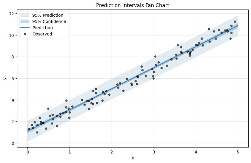
UQ visualization: fan charts, forest plots, BMA weights.#
%matplotlib inline
import matplotlib.pyplot as plt
from jaxsr.plotting import (
    plot_bma_weights,
    plot_coefficient_intervals,
    plot_prediction_intervals,
)

np.random.seed(42)
X = np.random.uniform(0, 5, (100, 1))
y = 2.0 * X[:, 0] + 1.0 + np.random.randn(100) * 0.5

library = (
    BasisLibrary(n_features=1, feature_names=["x"])
    .add_constant()
    .add_linear()
    .add_polynomials(max_degree=3)
)

model = SymbolicRegressor(
    basis_library=library,
    max_terms=4,
    strategy="greedy_forward",
)
model.fit(jnp.array(X), jnp.array(y))

X_plot = jnp.linspace(0, 5, 100).reshape(-1, 1)
fig, ax = plt.subplots(figsize=(10, 6))

# Plot smooth prediction/confidence bands using evenly-spaced X_plot
plot_prediction_intervals(model, X_plot, alpha=0.05, ax=ax)

# Overlay observed data at their actual x locations
ax.scatter(
    np.array(X[:, 0]),
    np.array(y),
    c="black",
    s=20,
    alpha=0.6,
    zorder=5,
    label="Observed",
)
ax.legend()
ax.set_title("Prediction Intervals Fan Chart")
plt.show()
ax = plot_coefficient_intervals(model)
plt.show()
ax = plot_bma_weights(model)
plt.show()