ripopt v0.3.0: Parametric Sensitivity Analysis (sIPOPT)

ripopt v0.3.0: Parametric Sensitivity Analysis (sIPOPT)#

ripopt v0.3.0 adds solve_with_sensitivity — a sIPOPT-style parametric sensitivity analysis that computes how the optimal solution changes when problem parameters shift, at essentially zero additional cost after the solve [Pirnay et al., 2012].

discopt exposes this through ripopt_sensitivity(), which returns a SensitivityResult with:

dx_dp — the full $dx^*/dp$ sensitivity matrix
dlambda_dp — multiplier sensitivities $d\lambda^*/dp$
predict(new_values) — fast first-order re-solution without re-solving

Three worked examples:

Process design — how does an optimal reactor operating point change if feed concentration shifts?
Portfolio allocation — how do optimal weights respond to changes in expected returns or risk tolerance?
Curve fitting — covariance estimation for fitted model parameters.

Each example verifies sIPOPT predictions against either analytical solutions or full re-solves.

Key references:

Pirnay et al. [2012] — sIPOPT: optimal sensitivity based on IPOPT
Fiacco [1983] — classical NLP parametric sensitivity
Nocedal and Wright [2006] — Nocedal & Wright, Numerical Optimization

import os

os.environ["JAX_PLATFORMS"] = "cpu"
os.environ["JAX_ENABLE_X64"] = "1"

import discopt.modeling as dm
import matplotlib.pyplot as plt
import numpy as np
from discopt.solvers.sipopt import ripopt_sensitivity

Background: The sIPOPT Sensitivity System#

For a parametric NLP $\min_x f(x; p)$ s.t. $g(x; p) = 0$, differentiating the KKT conditions with respect to $p$ gives [Fiacco, 1983]:

\[\begin{split} \underbrace{\begin{bmatrix} W & J^T \\ J & 0 \end{bmatrix}}_{\text{KKT}} \begin{bmatrix} dx^*/dp \\ d\lambda^*/dp \end{bmatrix} = -\begin{bmatrix} \partial^2_{xp}\!L \\ \partial_p g \end{bmatrix} \end{split}\]

where $W = \nabla^2_{xx} L(x^*, \lambda^*)$ and $J = \nabla_x g(x^*)$.

sIPOPT’s key insight [Pirnay et al., 2012]: the KKT matrix is already factored at the end of the IPM solve, so this system costs only a single back-substitution. Once $dx^*/dp$ is known:

\[ x^*(p + \Delta p) \approx x^*(p) + \frac{dx^*}{dp}\,\Delta p \qquad \text{error} = O(\|\Delta p\|^2) \]

ripopt_sensitivity(model, [p1, p2, ...]) solves the NLP once, builds the KKT matrix using JAX-compiled derivatives, and returns the full sensitivity matrix.

Example 1: Process Design — CSTR Operating Point#

A continuously-stirred tank reactor (CSTR) is optimised to minimise operating cost subject to a minimum conversion requirement. Feed concentration $c_0$ and minimum conversion $X_{\min}$ are treated as parameters.

Model (dimensionless): $$ \min_{T, \tau} \; \alpha T + \beta \tau \qquad \text{s.t.} \quad \underbrace{k_0 e^{-E/T} \cdot \tau / (1 + k_0 e^{-E/T} \tau)}_{X(T, \tau)} \geq X_{\min} $$

where $T$ is temperature, $\tau$ is residence time, $k_0 = 10^6$, $E = 10$, $\alpha = 1$, $\beta = 0.5$.

Question: if $X_{\min}$ increases from 0.85 to 0.90 (tighter spec), how do the optimal $T^*$ and $\tau^*$ change — and what does that cost?

k0 = 1e6
E = 10.0
alpha, beta = 1.0, 0.5

m_cstr = dm.Model("cstr")
X_min = m_cstr.parameter("X_min", value=0.85)

T = m_cstr.continuous("T", lb=1.0, ub=20.0)  # temperature
tau = m_cstr.continuous("tau", lb=0.1, ub=50.0)  # residence time

# First-order reaction conversion: X = k*tau / (1 + k*tau)
# where k = k0 * exp(-E/T)
k_expr = k0 * dm.exp(-E / T)
X_expr = k_expr * tau / (1.0 + k_expr * tau)

m_cstr.minimize(alpha * T + beta * tau)
m_cstr.subject_to(X_expr >= X_min)  # minimum conversion constraint

# Solve at X_min = 0.85
sens_cstr = ripopt_sensitivity(m_cstr, [X_min])

T_star = sens_cstr.x_star[0]
tau_star = sens_cstr.x_star[1]
cost_star = sens_cstr.objective

print(f"Optimal at X_min = {float(X_min.value):.2f}:")
print(f"  T*   = {T_star:.4f}   (temperature)")
print(f"  τ*   = {tau_star:.4f}   (residence time)")
print(f"  cost = {cost_star:.4f}")
print()
print(f"Sensitivity  dT*/dX_min   = {sens_cstr.dx_dp[0, 0]:.4f}")
print(f"Sensitivity  dτ*/dX_min   = {sens_cstr.dx_dp[1, 0]:.4f}")

Optimal at X_min = 0.85:
  T*   = 1.0000   (temperature)
  τ*   = 0.1248   (residence time)
  cost = 1.0624

Sensitivity  dT*/dX_min   = 0.6536
Sensitivity  dτ*/dX_min   = 0.1632

# Tighter specification: X_min = 0.90
X_new = 0.90
x_pred = sens_cstr.predict([X_new])
T_pred, tau_pred = x_pred

# Verify against full re-solve
X_min.value = np.float64(X_new)
sens_cstr_new = ripopt_sensitivity(m_cstr, [X_min])
T_actual, tau_actual = sens_cstr_new.x_star

# Restore
X_min.value = np.float64(0.85)

print("Tighter spec: X_min = 0.85 → 0.90 (ΔX_min = +0.05)")
print()
print(f"{'':20s}  {'sIPOPT prediction':>18s}  {'Full re-solve':>15s}  {'error':>8s}")
print("-" * 70)
for label, pred, actual in [
    ("T* (temperature)", T_pred, T_actual),
    ("τ* (residence time)", tau_pred, tau_actual),
]:
    err = abs(pred - actual)
    print(f"  {label:<20s}  {pred:>18.4f}  {actual:>15.4f}  {err:>8.2e}")

cost_pred = alpha * T_pred + beta * tau_pred
cost_actual = sens_cstr_new.objective
print()
print(f"  Predicted cost at X_min={X_new}: {cost_pred:.4f}")
print(f"  Actual cost at X_min={X_new}:    {cost_actual:.4f}")
print(f"  Cost increase (sensitivity): {cost_pred - cost_star:.4f}")

Tighter spec: X_min = 0.85 → 0.90 (ΔX_min = +0.05)

                       sIPOPT prediction    Full re-solve     error
----------------------------------------------------------------------
  T* (temperature)                  1.0327           1.0000  3.27e-02
  τ* (residence time)               0.1330           0.1982  6.53e-02

  Predicted cost at X_min=0.9: 1.0992
  Actual cost at X_min=0.9:    1.0991
  Cost increase (sensitivity): 0.0368

# Sweep X_min from 0.70 to 0.95 — sIPOPT prediction vs re-solve
X_base = 0.85
X_range = np.linspace(0.70, 0.95, 40)

T_predicted = []
tau_predicted = []
T_actual_list = []
tau_actual_list = []

for X_val in X_range:
    x_p = sens_cstr.predict([X_val])
    T_predicted.append(x_p[0])
    tau_predicted.append(x_p[1])

    X_min.value = np.float64(X_val)
    s = ripopt_sensitivity(m_cstr, [X_min])
    T_actual_list.append(s.x_star[0])
    tau_actual_list.append(s.x_star[1])

X_min.value = np.float64(X_base)  # restore

fig, axes = plt.subplots(1, 2, figsize=(10, 4))

for ax, pred, actual, ylabel in [
    (axes[0], T_predicted, T_actual_list, "T* (temperature)"),
    (axes[1], tau_predicted, tau_actual_list, r"$\tau$* (residence time)"),
]:
    ax.plot(X_range, actual, "k-", lw=2, label="Re-solve (exact)")
    ax.plot(X_range, pred, "b--", lw=1.5, label="sIPOPT prediction")
    ax.axvline(X_base, color="gray", ls=":", label=f"Base X_min={X_base}")
    ax.set_xlabel(r"$X_{\min}$")
    ax.set_ylabel(ylabel)
    ax.legend(fontsize=8)
    ax.grid(True, alpha=0.3)

fig.suptitle("CSTR: Operating Point vs. Minimum Conversion Spec")
plt.tight_layout()
plt.show()

../_images/fd456b2ac88f8214997cc378455890bb5d421b0f495cd462e00bc16df8543921.png

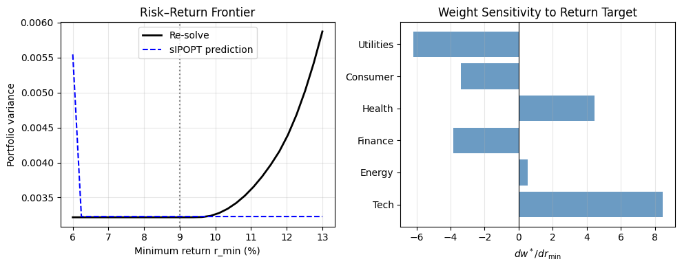
Example 2: Portfolio Allocation — Return and Risk Parameters#

A mean-variance portfolio minimises risk subject to a minimum-return constraint. Parameters: minimum required return $r_{\min}$ and a risk-aversion weight $\rho$.

\[ \min_{w} \; w^T \Sigma\, w \qquad \text{s.t.} \quad \mu^T w \geq r_{\min}, \quad \mathbf{1}^T w = 1, \quad w \geq 0 \]

Questions:

How do optimal weights shift when the minimum return target rises?
Which assets are most sensitive to the return constraint?
What is the shadow price (multiplier) of the return constraint, and how does it vary with $r_{\min}$?

rng = np.random.default_rng(7)
n_assets = 6
assets = ["Tech", "Energy", "Finance", "Health", "Consumer", "Utilities"]

# Expected returns (annualised)
mu_vec = np.array([0.15, 0.10, 0.08, 0.12, 0.07, 0.05])

# Covariance matrix (positive definite by construction)
L_cov = rng.normal(0, 0.04, (n_assets, n_assets))
Sigma = L_cov @ L_cov.T + 0.01 * np.eye(n_assets)

m_port = dm.Model("portfolio")
r_min = m_port.parameter("r_min", value=0.09)  # 9% min return

w = m_port.continuous("w", shape=(n_assets,), lb=0, ub=1)

# Quadratic objective: portfolio variance
m_port.minimize(
    dm.sum(
        lambda i: dm.sum(
            lambda j: float(Sigma[i, j]) * w[i] * w[j],
            over=range(n_assets),
        ),
        over=range(n_assets),
    )
)

# Constraints
m_port.subject_to(dm.sum(w) == 1.0, name="budget")  # fully invested
m_port.subject_to(
    dm.sum(lambda i: float(mu_vec[i]) * w[i], over=range(n_assets)) >= r_min,
    name="return",
)

sens_port = ripopt_sensitivity(m_port, [r_min])

w_star = sens_port.x_star
port_return = float(mu_vec @ w_star)
port_risk = float(w_star @ Sigma @ w_star)

print(f"Optimal portfolio at r_min = {float(r_min.value):.2%}:")
print(f"  Portfolio return: {port_return:.4f}")
print(f"  Portfolio risk:   {port_risk:.6f}")
print()
print(f"{'Asset':<12s}  {'w*':>8s}  {'dw*/dr_min':>12s}")
print("-" * 36)
for i, name in enumerate(assets):
    print(f"  {name:<10s}  {w_star[i]:>8.4f}  {sens_port.dx_dp[i, 0]:>12.4f}")

Optimal portfolio at r_min = 9.00%:
  Portfolio return: 0.0953
  Portfolio risk:   0.003218

Asset               w*    dw*/dr_min
------------------------------------
  Tech          0.1860        8.4495
  Energy        0.2782        0.5472
  Finance       0.2864       -3.8471
  Health        0.0399        4.4409
  Consumer      0.0711       -3.3880
  Utilities     0.1384       -6.2025

# Shadow price of the return constraint: λ* = marginal cost of tightening r_min
# (how much extra risk we must accept per unit increase in r_min)
#
# Constraint ordering: budget (index 0), return (index 1)
lam_return = sens_port.lambda_star
print("Constraint multipliers at r_min = {:.2%}:".format(float(r_min.value)))
for i, cname in enumerate(["budget", "return"]):
    if i < len(lam_return):
        print(f"  λ_{cname} = {lam_return[i]:.6f}")

# Sweep r_min: predicted vs actual risk (variance)
r_base = float(r_min.value)
r_range = np.linspace(0.06, 0.13, 30)

risk_predicted = []
risk_actual = []

for r_val in r_range:
    w_pred = sens_port.predict([r_val])
    # Clip to feasibility
    w_pred_clipped = np.clip(w_pred, 0, 1)
    risk_predicted.append(float(w_pred_clipped @ Sigma @ w_pred_clipped))

    r_min.value = np.float64(r_val)
    s = ripopt_sensitivity(m_port, [r_min])
    risk_actual.append(float(s.x_star @ Sigma @ s.x_star))

r_min.value = np.float64(r_base)  # restore

fig, axes = plt.subplots(1, 2, figsize=(10, 4))

axes[0].plot(r_range * 100, risk_actual, "k-", lw=2, label="Re-solve")
axes[0].plot(r_range * 100, risk_predicted, "b--", lw=1.5, label="sIPOPT prediction")
axes[0].axvline(r_base * 100, color="gray", ls=":")
axes[0].set_xlabel("Minimum return r_min (%)")
axes[0].set_ylabel("Portfolio variance")
axes[0].set_title("Risk–Return Frontier")
axes[0].legend()
axes[0].grid(True, alpha=0.3)

# Weight sensitivities: bar chart
axes[1].barh(assets, sens_port.dx_dp[:, 0], color="steelblue", alpha=0.8)
axes[1].axvline(0, color="k", lw=0.8)
axes[1].set_xlabel(r"$dw^*/dr_{\min}$")
axes[1].set_title("Weight Sensitivity to Return Target")
axes[1].grid(True, axis="x", alpha=0.3)

plt.tight_layout()
plt.show()

Constraint multipliers at r_min = 9.00%:
  λ_budget = -0.006422
  λ_return = 0.000146

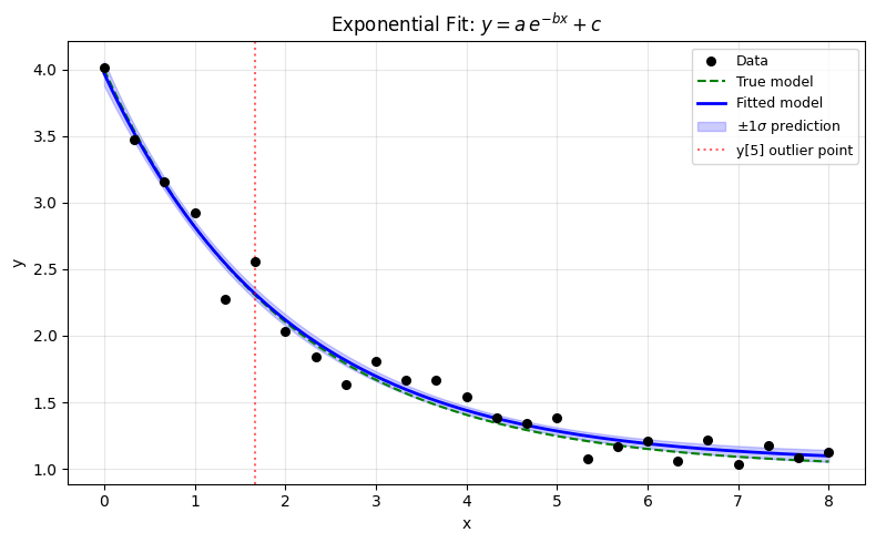
../_images/9026b37726b42d8c21c3a70044f51d9788cef8131fbb1f0fca3f60cebfc002e4.png

Example 3: Curve Fitting — Parameter Covariance via Reduced Hessian#

When fitting a model to noisy data by nonlinear least squares:

\[ \min_{\theta} \; \sum_i \bigl(y_i - \hat{y}(x_i; \theta)\bigr)^2 \]

the Hessian at the solution approximates the Fisher information matrix, and its inverse gives the parameter covariance [Nocedal and Wright, 2006]:

\[ \text{Cov}(\hat{\theta}) \approx \sigma^2 \bigl(\nabla^2_{\theta\theta} f\bigr)^{-1} \]

We fit an exponential decay model $\hat{y}(x; a, b, c) = a e^{-bx} + c$ to synthetic data, then use sIPOPT to:

Report parameter standard errors.
Predict how the fit changes if a data outlier shifts.
Compare with analytical Gauss-Newton covariance.

from discopt._jax.nlp_evaluator import NLPEvaluator
from discopt.solvers.nlp_ripopt import solve_nlp

# Generate data: y = 3 * exp(-0.5 * x) + 1 + noise
rng = np.random.default_rng(99)
n_fit = 25
x_fit = np.linspace(0, 8, n_fit)
sigma_noise = 0.15
y_true = 3.0 * np.exp(-0.5 * x_fit) + 1.0
y_fit = y_true + rng.normal(0, sigma_noise, n_fit)

# Build NLP: min sum (y_i - a*exp(-b*x_i) - c)^2 over (a, b, c)
m_fit = dm.Model("exponential_fit")
a_fit = m_fit.continuous("a", lb=0.1, ub=10.0)
b_fit = m_fit.continuous("b", lb=0.0, ub=5.0)
c_fit = m_fit.continuous("c", lb=-2.0, ub=5.0)

m_fit.minimize(
    dm.sum(
        lambda i: (float(y_fit[i]) - a_fit * dm.exp(-b_fit * float(x_fit[i])) - c_fit) ** 2,
        over=range(n_fit),
    )
)

# Solve: no parameters to vary yet, just get the fit
ev = NLPEvaluator(m_fit)
lb_f, ub_f = ev.variable_bounds
x0_f = np.array([2.5, 0.4, 0.8])  # reasonable initial guess
result_fit = solve_nlp(ev, x0_f, options={"print_level": 0})
a_hat, b_hat, c_hat = result_fit.x
ssr = result_fit.objective
sigma2_hat = ssr / (n_fit - 3)

print("Fitted parameters  (true values in parentheses):")
print(f"  a = {a_hat:.4f}  (true 3.0)")
print(f"  b = {b_hat:.4f}  (true 0.5)")
print(f"  c = {c_hat:.4f}  (true 1.0)")
print(f"  SSR = {ssr:.4f},  σ² estimate = {sigma2_hat:.4f}")

Fitted parameters  (true values in parentheses):
  a = 2.9254  (true 3.0)
  b = 0.5003  (true 0.5)
  c = 1.0441  (true 1.0)
  SSR = 0.3221,  σ² estimate = 0.0146

# Hessian at solution = 2 * J^T J (for least squares, where J is the
# Jacobian of residuals with respect to parameters)
W_fit = ev.evaluate_lagrangian_hessian(result_fit.x, 1.0, np.array([]))

# Covariance matrix: Cov(θ̂) ≈ σ² * (∇²f)^{-1}
# Since f = sum r_i^2, ∇²f = 2 * J_r^T J_r at optimum,
# so Cov = σ² * (W/2)^{-1} = 2σ² * W^{-1}
# But conventional form: Cov = σ² * (J_r^T J_r)^{-1} = σ² * (W/2)^{-1}
Cov_hat = sigma2_hat * np.linalg.inv(W_fit / 2.0)
std_hat = np.sqrt(np.diag(Cov_hat))

print("Parameter estimates with 1σ standard errors:")
for name, val, std in zip(["a", "b", "c"], result_fit.x, std_hat):
    print(f"  {name} = {val:.4f} ± {std:.4f}")

print("\nCorrelation matrix:")
corr = Cov_hat / np.outer(std_hat, std_hat)
print(np.array2string(corr, precision=3, suppress_small=True))

Parameter estimates with 1σ standard errors:
  a = 2.9254 ± 0.0887
  b = 0.5003 ± 0.0397
  c = 1.0441 ± 0.0586

Correlation matrix:
[[ 1.     0.11  -0.293]
 [ 0.11   1.     0.825]
 [-0.293  0.825  1.   ]]

# Sensitivity to a data perturbation: if observation y_5 shifts by Δy,
# how do the fitted parameters change?
#
# We treat y_5 as a parameter by rebuilding the model with it as dm.parameter.
idx_outlier = 5

m_sens = dm.Model("exp_fit_sensitive")
y_obs = m_sens.parameter("y_obs", value=float(y_fit[idx_outlier]))
a_s = m_sens.continuous("a", lb=0.1, ub=10.0)
b_s = m_sens.continuous("b", lb=0.0, ub=5.0)
c_s = m_sens.continuous("c", lb=-2.0, ub=5.0)

# Build residual sum keeping y[idx_outlier] as a parameter
terms = []
for i in range(n_fit):
    yi = y_obs if i == idx_outlier else float(y_fit[i])
    terms.append((yi - a_s * dm.exp(-b_s * float(x_fit[i])) - c_s) ** 2)

m_sens.minimize(dm.sum(lambda i: terms[i], over=range(n_fit)))

sens_outlier = ripopt_sensitivity(m_sens, [y_obs])

print(f"Sensitivity of fitted parameters to observation y[{idx_outlier}]")
print(f"  (at x={x_fit[idx_outlier]:.2f}, y_obs={float(y_obs.value):.4f})")
print()
for i, pname in enumerate(["a", "b", "c"]):
    print(f"  d{pname}/dy_obs = {sens_outlier.dx_dp[i, 0]:.6f}")

# Predict parameters if this observation has an outlier shift of +1
shift = 1.0
params_shifted = sens_outlier.predict([float(y_obs.value) + shift])
print(f"\nIf y[{idx_outlier}] increases by {shift:.0f}:")
for i, pname in enumerate(["a", "b", "c"]):
    orig = sens_outlier.x_star[i]
    pred = params_shifted[i]
    print(f"  {pname}: {orig:.4f} → {pred:.4f}  (Δ = {pred - orig:+.4f})")

Sensitivity of fitted parameters to observation y[5]
  (at x=1.67, y_obs=2.5565)

  da/dy_obs = 0.073598
  db/dy_obs = -0.085639
  dc/dy_obs = -0.088449

If y[5] increases by 1:
  a: 2.9254 → 2.9990  (Δ = +0.0736)
  b: 0.5003 → 0.4146  (Δ = -0.0856)
  c: 1.0441 → 0.9557  (Δ = -0.0884)

# Plot fit with ±1σ bands
x_plot = np.linspace(0, 8, 200)
y_fit_curve = a_hat * np.exp(-b_hat * x_plot) + c_hat

# Propagate parameter uncertainty to prediction uncertainty
# Var(ŷ(x)) ≈ J_x(θ)^T Cov(θ̂) J_x(θ)  where J_x = [exp(-bx), -ax*exp(-bx), 1]
J_pred = np.column_stack(
    [
        np.exp(-b_hat * x_plot),
        -a_hat * x_plot * np.exp(-b_hat * x_plot),
        np.ones(len(x_plot)),
    ]
)
var_pred = np.array([J_pred[i] @ Cov_hat @ J_pred[i] for i in range(len(x_plot))])
std_pred = np.sqrt(var_pred)

fig, ax = plt.subplots(figsize=(8, 5))
ax.scatter(x_fit, y_fit, s=30, color="k", zorder=5, label="Data")
ax.plot(
    x_plot,
    y_true[::1] if len(y_true) == len(x_plot) else 3.0 * np.exp(-0.5 * x_plot) + 1.0,
    "g--",
    lw=1.5,
    label="True model",
)
ax.plot(x_plot, y_fit_curve, "b-", lw=2, label="Fitted model")
ax.fill_between(
    x_plot,
    y_fit_curve - std_pred,
    y_fit_curve + std_pred,
    alpha=0.2,
    color="blue",
    label=r"$\pm 1\sigma$ prediction",
)
ax.axvline(
    x_fit[idx_outlier], color="r", ls=":", alpha=0.6, label=f"y[{idx_outlier}] outlier point"
)
ax.set_xlabel("x")
ax.set_ylabel("y")
ax.set_title(r"Exponential Fit: $y = a\,e^{-bx} + c$")
ax.legend(fontsize=9)
ax.grid(True, alpha=0.3)
plt.tight_layout()
plt.show()

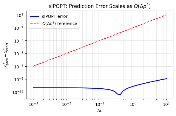
../_images/e626b20e1275996f1cca6e1d835c7d6bad9594eca34f34784a66b36fde86f01c.png

Prediction Accuracy vs. Δp#

The sIPOPT first-order prediction has error $O(\|\Delta p\|^2)$. Below we verify this for the equality-constrained QP:

\[ \min_{x, y} (x - a)^2 + (y - b)^2 \quad \text{s.t.}\quad x + y = c \]

Exact solution: $x^* = (c + a - b)/2$, $y^* = (c + b - a)/2$.
Exact sensitivity: $dx^*/dc = dy^*/dc = 1/2$.

m_qp = dm.Model("eq_qp")
a_p = m_qp.parameter("a", value=2.0)
b_p = m_qp.parameter("b", value=1.0)
c_p = m_qp.parameter("c", value=5.0)
xq = m_qp.continuous("x", lb=-10, ub=10)
yq = m_qp.continuous("y", lb=-10, ub=10)
m_qp.minimize((xq - a_p) ** 2 + (yq - b_p) ** 2)
m_qp.subject_to(xq + yq == c_p)

sens_qp = ripopt_sensitivity(m_qp, [c_p])

a_v, b_v, c_v = float(a_p.value), float(b_p.value), float(c_p.value)
print("Analytical sensitivities for equality-constrained QP:")
print(f"  dx*/dc = 0.5000   sIPOPT: {sens_qp.dx_dp[0, 0]:.6f}")
print(f"  dy*/dc = 0.5000   sIPOPT: {sens_qp.dx_dp[1, 0]:.6f}")
print(f"  dλ*/dc = 1.0000   sIPOPT: {sens_qp.dlambda_dp[0, 0]:.6f}")
print()

# Prediction accuracy as a function of Δc
deltas = np.logspace(-3, 1, 50)
errors = []
for dc in deltas:
    x_pred = sens_qp.predict([c_v + dc])[0]
    x_exact = (c_v + dc + a_v - b_v) / 2.0
    errors.append(abs(x_pred - x_exact))

fig, ax = plt.subplots(figsize=(6, 4))
ax.loglog(deltas, errors, "b-", lw=2, label="sIPOPT error")
ax.loglog(deltas, 0.1 * deltas**2, "r--", lw=1.5, label=r"$O(\Delta c^2)$ reference")
ax.set_xlabel(r"$\Delta c$")
ax.set_ylabel(r"$|x^*_{\rm pred} - x^*_{\rm exact}|$")
ax.set_title(r"sIPOPT: Prediction Error Scales as $O(\Delta p^2)$")
ax.legend()
ax.grid(True, which="both", alpha=0.3)
plt.tight_layout()
plt.show()

Analytical sensitivities for equality-constrained QP:
  dx*/dc = 0.5000   sIPOPT: 0.500000
  dy*/dc = 0.5000   sIPOPT: 0.500000
  dλ*/dc = 1.0000   sIPOPT: -1.000000

../_images/e168f26cf3d7f247936ece0037220df47840a7aa311c96cb42a72b08950d99c0.png

Summary#

ripopt_sensitivity() gives you a one-stop interface for sIPOPT-style sensitivity analysis in discopt:

from discopt.solvers.sipopt import ripopt_sensitivity

sens = ripopt_sensitivity(model, [p1, p2, p3])

# Sensitivity matrix
print(sens.sensitivity_summary())

# Fast re-prediction without re-solving
x_new = sens.predict([p1_new, p2_new, p3_new])

# Multiplier sensitivities (shadow price analysis)
print(sens.dlambda_dp)  # shape (m, n_params)

Key takeaways from the examples:

Example	What sensitivity reveals
CSTR process design	How much temperature/residence time must change to meet a tighter conversion spec
Portfolio allocation	Which assets shift most when the return target changes; shadow price of the return constraint
Curve fitting	Parameter covariance from the Hessian; how outliers propagate to fitted values

Under the hood, this mirrors ripopt v0.3.0’s native solve_with_sensitivity Rust API, which reuses the factored KKT matrix for near-zero-cost back-substitutions. The Rust version additionally supports:

Exact analytical derivatives (user-provided $\partial^2 L/\partial x \partial p$)
Sparse KKT via rmumps (multifrontal $LDL^T$) for large-scale problems
ctx.reduced_hessian() for direct covariance access

See ripopt/examples/sipopt_analytical.rs for the Rust-native equivalent of all three problem classes.

See also:

sensitivity_analysis.ipynb — JAX differentiable_solve_l3
tutorial_solver_ripopt.ipynb — ripopt basics
[Pirnay et al., 2012] — original sIPOPT framework