Model-Based Design of Experiments

This tutorial demonstrates how to use discopt.doe for optimal experimental design. The key idea: given a model with unknown parameters, find the experimental conditions that maximize the information we can extract about those parameters [Franceschini and Macchietto, 2008].

Key advantage over Pyomo.DoE [Wang and Dowling, 2022]: discopt computes the sensitivity Jacobian \(\partial y / \partial \theta\) via exact JAX autodiff rather than finite differences. This gives:

• No step-size tuning

• No truncation error

• No extra model solves (Pyomo.DoE needs \(2N\) extra solves for central differences)

Contents:

1. Fisher Information Matrix (FIM) computation

2. Design space exploration

3. Optimal experimental design

4. Sequential DoE loop

5. Identifiability analysis

import os

os.environ["JAX_PLATFORMS"] = "cpu"
os.environ["JAX_ENABLE_X64"] = "1"

import discopt.modeling as dm
import matplotlib.pyplot as plt
import numpy as np
from discopt.doe import (
    DesignCriterion,
    check_identifiability,
    compute_fim,
    explore_design_space,
    optimal_experiment,
    sequential_doe,
)
from discopt.estimate import Experiment, ExperimentModel

1. Fisher Information Matrix

The FIM quantifies how much information an experiment provides about unknown parameters. For a model with responses \(y = f(\theta, d)\) and measurement error covariance \(\Sigma\):

\[\text{FIM} = J^T \Sigma^{-1} J\]

where \(J_{ij} = \partial y_i / \partial \theta_j\) is the sensitivity Jacobian. A larger FIM means more information and tighter parameter confidence intervals (\(\text{Cov}(\theta) \approx \text{FIM}^{-1}\)).

Design criteria [Atkinson et al., 2007]

Criterion	Objective	Interpretation
D-optimal	max \(\log \det(\text{FIM})\)	Minimize volume of confidence ellipsoid
A-optimal	min \(\text{tr}(\text{FIM}^{-1})\)	Minimize average variance
E-optimal	max \(\lambda_{\min}(\text{FIM})\)	Minimize worst-case variance
ME-optimal	min \(\kappa(\text{FIM})\)	Balance information across parameters

class MeasurementExperiment(Experiment):
    """y = k * x at a single design point x. Estimate k."""

    def create_model(self, **kwargs):
        m = dm.Model("measurement")
        k = m.continuous("k", lb=0.01, ub=20)
        x = m.continuous("x", lb=0.1, ub=10)
        return ExperimentModel(
            model=m,
            unknown_parameters={"k": k},
            design_inputs={"x": x},
            responses={"y": k * x},
            measurement_error={"y": 0.1},
        )


exp = MeasurementExperiment()

# Compute FIM at two different design points
fim_low = compute_fim(exp, {"k": 2.0}, {"x": 1.0})
fim_high = compute_fim(exp, {"k": 2.0}, {"x": 10.0})

print(f"FIM at x=1:  {fim_low.fim[0, 0]:.1f}  (D-opt: {fim_low.d_optimal:.2f})")
print(f"FIM at x=10: {fim_high.fim[0, 0]:.1f}  (D-opt: {fim_high.d_optimal:.2f})")
print("\nFor y=k*x: FIM = x^2/sigma^2, so x=10 gives 100x more information.")

FIM at x=1:  100.0  (D-opt: 4.61)
FIM at x=10: 10000.0  (D-opt: 9.21)

For y=k*x: FIM = x^2/sigma^2, so x=10 gives 100x more information.

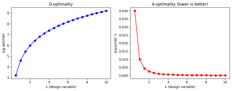
2. Design space exploration

Before optimizing, it’s useful to visualize how the FIM criteria vary across the design space.

result = explore_design_space(
    exp,
    param_values={"k": 2.0},
    design_ranges={"x": np.linspace(0.5, 10.0, 20)},
)

fig, axes = plt.subplots(1, 2, figsize=(10, 4))
axes[0].plot(result.grid["x"], result.metrics["log_det_fim"], "bo-")
axes[0].set_xlabel("x (design variable)")
axes[0].set_ylabel("log det(FIM)")
axes[0].set_title("D-optimality")

axes[1].plot(result.grid["x"], result.metrics["trace_fim_inv"], "ro-")
axes[1].set_xlabel("x (design variable)")
axes[1].set_ylabel("trace(FIM⁻¹)")
axes[1].set_title("A-optimality (lower is better)")
plt.tight_layout();

3. Optimal experimental design

optimal_experiment() finds the design that maximizes the chosen criterion.

design = optimal_experiment(
    exp,
    param_values={"k": 2.0},
    design_bounds={"x": (0.5, 10.0)},
    criterion=DesignCriterion.D_OPTIMAL,
)

print(design.summary())

Optimal Experimental Design
==================================================
                x = 10

  D-opt (log det FIM) = 9.21
  A-opt (trace FIM⁻¹) = 0.0001
  E-opt (min eigenval) = 1e+04
  Condition number     = 1

  SE(k) = 0.01

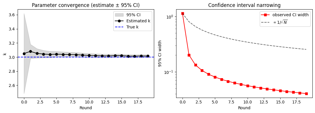
4. Sequential DoE

The most powerful workflow: alternate between estimating parameters and designing the next experiment. Each round accumulates information.

class MultiPointExperiment(Experiment):
    """y_i = k * x_i at multiple measurement points."""

    def __init__(self, x_data):
        self.x_data = x_data

    def create_model(self, **kwargs):
        m = dm.Model("multi")
        k = m.continuous("k", lb=0.01, ub=20)
        responses, errors = {}, {}
        for i, xi in enumerate(self.x_data):
            responses[f"y_{i}"] = k * xi
            errors[f"y_{i}"] = 0.1
        return ExperimentModel(
            model=m,
            unknown_parameters={"k": k},
            design_inputs={},
            responses=responses,
            measurement_error=errors,
        )


# Start with 2 noisy measurements.
k_true = 3.0
x_pts = np.array([1.0, 2.0])
exp_multi = MultiPointExperiment(x_pts)
np.random.seed(0)
initial_data = {f"y_{i}": k_true * x_pts[i] + 0.1 * np.random.randn() for i in range(len(x_pts))}


# Synthetic experiment runner: re-measures the same design points each round
# (the Experiment has no design inputs here, so sequential_doe is just
# repeated sampling + incremental re-estimation).
def run_exp(design):
    return {f"y_{i}": k_true * x_pts[i] + 0.1 * np.random.randn() for i in range(len(x_pts))}


history = sequential_doe(
    experiment=exp_multi,
    initial_data=initial_data,
    initial_guess={"k": 1.0},
    design_bounds={},
    n_rounds=20,
    run_experiment=run_exp,
)

rounds = np.array([r.round for r in history])
estimates = np.array([r.estimation.parameters["k"] for r in history])
ci_lo = np.array([r.estimation.confidence_intervals["k"][0] for r in history])
ci_hi = np.array([r.estimation.confidence_intervals["k"][1] for r in history])

fig, axes = plt.subplots(1, 2, figsize=(11, 4))

# Left: estimate with 95% CI band; true value inside the band at every round.
axes[0].fill_between(rounds, ci_lo, ci_hi, color="k", alpha=0.15, label="95% CI")
axes[0].plot(rounds, estimates, "ko-", label="Estimated k")
axes[0].axhline(k_true, color="b", ls="--", label="True k")
axes[0].set_xlabel("Round")
axes[0].set_ylabel("k")
axes[0].legend()
axes[0].set_title("Parameter convergence (estimate ± 95% CI)")

# Right: CI width on a log scale -- should decay like 1/sqrt(N).
axes[1].semilogy(rounds, ci_hi - ci_lo, "rs-", label="observed CI width")
# Reference curve: width ∝ 1/sqrt(total observations).
n_obs = np.array([r.estimation.n_observations for r in history])
ref = (ci_hi[0] - ci_lo[0]) * np.sqrt(n_obs[0] / n_obs)
axes[1].semilogy(rounds, ref, "k--", alpha=0.6, label=r"$\propto 1/\sqrt{N}$")
axes[1].set_xlabel("Round")
axes[1].set_ylabel("95% CI width")
axes[1].set_title("Confidence interval narrowing")
axes[1].legend()

plt.tight_layout();

5. Identifiability analysis

Before running experiments, check that your parameters are structurally identifiable from the proposed measurements.

# Identifiable: y = a*x + b (2 params, multiple measurements)
class LinearExperiment(Experiment):
    def create_model(self, **kwargs):
        m = dm.Model("linear")
        a = m.continuous("a", lb=-10, ub=10)
        b = m.continuous("b", lb=-10, ub=10)
        return ExperimentModel(
            model=m,
            unknown_parameters={"a": a, "b": b},
            design_inputs={},
            responses={"y1": a * 1.0 + b, "y2": a * 2.0 + b},
            measurement_error={"y1": 0.1, "y2": 0.1},
        )


r1 = check_identifiability(LinearExperiment(), {"a": 1.0, "b": 0.0})
print(f"Linear model: identifiable={r1.is_identifiable}, rank={r1.fim_rank}/{r1.n_parameters}")


# Unidentifiable: y = (a*b)*x (product of 2 params)
class ProductExperiment(Experiment):
    def create_model(self, **kwargs):
        m = dm.Model("product")
        a = m.continuous("a", lb=0.1, ub=10)
        b = m.continuous("b", lb=0.1, ub=10)
        return ExperimentModel(
            model=m,
            unknown_parameters={"a": a, "b": b},
            design_inputs={},
            responses={"y1": a * b * 1.0, "y2": a * b * 2.0},
            measurement_error={"y1": 0.1, "y2": 0.1},
        )


r2 = check_identifiability(ProductExperiment(), {"a": 2.0, "b": 3.0})
print(f"Product model: identifiable={r2.is_identifiable}, rank={r2.fim_rank}/{r2.n_parameters}")
print(f"  Problematic parameters: {r2.problematic_parameters}")

Linear model: identifiable=True, rank=2/2
Product model: identifiable=False, rank=1/2
  Problematic parameters: ['b']

6. Autodiff vs finite differences

discopt computes exact Jacobians via JAX autodiff. Let’s compare accuracy against finite differences at various step sizes.

exp = MeasurementExperiment()
pv = {"k": 2.0}
dv = {"x": 5.0}

fim_exact = compute_fim(exp, pv, dv, method="autodiff")

steps = [1e-3, 1e-4, 1e-5, 1e-6, 1e-7, 1e-8]
errors = []
for step in steps:
    fim_fd = compute_fim(exp, pv, dv, method="finite_difference", fd_step=step)
    err = np.max(np.abs(fim_fd.fim - fim_exact.fim))
    errors.append(err)

plt.loglog(steps, errors, "ko-")
plt.xlabel("Finite difference step size")
plt.ylabel("Max absolute error in FIM")
plt.title("Autodiff is exact; FD accuracy depends on step size")
plt.grid(True);