Multi-Objective Optimization#
This tutorial shows how discopt.mo wraps discopt’s single-objective MINLP
solver in classical scalarization loops, producing a
ParetoFront approximation for problems with two or more conflicting
objectives.
A multi-objective problem replaces a single scalar objective with a vector \(F(x) = (f_1(x), \ldots, f_k(x))\). In general no \(x\) minimizes every \(f_i\) simultaneously; the solution concept is the Pareto front – the set of trade-offs where improving one objective requires worsening another [Miettinen, 1999] [Ehrgott, 2005].
discopt.mo exposes five deterministic scalarization methods:
Method |
API |
Complete on nonconvex fronts? |
|---|---|---|
Weighted sum |
|
|
AUGMECON2 \(\varepsilon\)-constraint |
|
Yes [Mavrotas, 2009] |
Augmented weighted Tchebycheff |
|
Yes [Steuer and Choo, 1983] |
Normal Boundary Intersection |
|
Yes [Das and Dennis, 1998] |
Normalized Normal Constraint |
|
Yes [Messac et al., 2003] |
Each returns a ParetoFront carrying the Pareto points, ideal/nadir
estimates, sense information, and helpers for indicators and plotting.
import os

os.environ["JAX_PLATFORMS"] = "cpu"
os.environ["JAX_ENABLE_X64"] = "1"

import discopt.modeling as dm
import matplotlib.pyplot as plt
import numpy as np
from discopt.mo import (
    epsilon_constraint,
    normal_boundary_intersection,
    normalized_normal_constraint,
    weighted_sum,
    weighted_tchebycheff,
)
1. A convex bi-objective MINLP#
We start with the canonical bi-objective convex QP
The Pareto front has the closed form \(\sqrt{f_1/5} + \sqrt{f_2/5} = 1\) and is convex, so every scalarization should recover it.
def build_convex_qp():
    m = dm.Model("biobj_qp")
    x = m.continuous("x", lb=-5, ub=5)
    y = m.continuous("y", lb=-5, ub=5)
    f1 = x**2 + y**2
    f2 = (x - 2) ** 2 + (y - 1) ** 2
    return m, [f1, f2]


# Analytic front for reference plotting.
alpha = np.linspace(0, 1, 101)
ref_f1 = 5 * alpha**2
ref_f2 = 5 * (1 - alpha) ** 2
1.1 Weighted sum#
The simplest scalarization is a convex combination \(\min \sum_i w_i f_i(x)\) with \(w\) ranging over the simplex. It recovers every Pareto point on a convex front but misses concave pieces.
m, objs = build_convex_qp()
front_ws = weighted_sum(m, objs, n_weights=11)
print(front_ws.summary())
Pareto Front (weighted_sum, 11 points, k=2)
============================================================
  ideal: f1=0, f2=1.332e-14
  nadir: f1=5, f2=5

            f1            f2
  ------------  ------------
             5     3.125e-13
          4.05     0.0500002
           3.2           0.2
          2.45      0.450001
           1.8      0.800001
          1.25          1.25
           0.8           1.8
          0.45          2.45
           0.2           3.2
          0.05          4.05
             0             5
1.2 AUGMECON2 (\(\varepsilon\)-constraint)#
Minimize one objective; bound the others by \(\varepsilon_i\) parameters. The augmented form (default) adds a non-negative slack per bound and a small slack-reward penalty so every returned point is strictly Pareto- optimal [Mavrotas, 2009].
m, objs = build_convex_qp()
front_eps = epsilon_constraint(m, objs, n_points=11)
print(front_eps.summary())
******************************************************************************
This program contains Ipopt, a library for large-scale nonlinear optimization.
 Ipopt is released as open source code under the Eclipse Public License (EPL).
         For more information visit https://github.com/coin-or/Ipopt
******************************************************************************
Pareto Front (augmecon2, 11 points, k=2)
============================================================
  ideal: f1=0, f2=1.332e-14
  nadir: f1=5, f2=5

            f1            f2
  ------------  ------------
       4.99937   1.99997e-08
       2.33772           0.5
       1.52786             1
       1.02277           1.5
      0.675445             2
      0.428932           2.5
      0.254033             3
        0.1334           3.5
     0.0557281             4
      0.013167           4.5
   2.01766e-07       4.99799
1.3 Weighted Tchebycheff#
Minimize the \(L_\infty\) distance from the ideal point under weights \(w\):
Unlike weighted sum, every Pareto-optimal point is attainable for some \(w\), with no convexity assumption [Steuer and Choo, 1983].
m, objs = build_convex_qp()
front_tch = weighted_tchebycheff(m, objs, n_weights=11)
print(front_tch.summary())
Pareto Front (weighted_tchebycheff, 11 points, k=2)
============================================================
  ideal: f1=0, f2=1.332e-14
  nadir: f1=5, f2=5

            f1            f2
  ------------  ------------
             5   6.79531e-18
        2.8125        0.3125
       2.22222      0.555556
       1.82623      0.782671
       1.51531       1.01021
          1.25          1.25
       1.01021       1.51531
      0.782671       1.82623
      0.555556       2.22222
        0.3125        2.8125
   1.23991e-41             5
1.4 NBI and NNC#
Normal Boundary Intersection [Das and Dennis, 1998] and the Normalized Normal Constraint method [Messac et al., 2003] are geometric scalarizations designed for uniform spacing of the returned points along the front, irrespective of curvature.
m, objs = build_convex_qp()
front_nbi = normal_boundary_intersection(m, objs, n_points=11)

m, objs = build_convex_qp()
front_nnc = normalized_normal_constraint(m, objs, n_points=11)

print("NBI:", front_nbi.n, "points,  NNC:", front_nnc.n, "points")
NBI: 11 points, NNC: 11 points
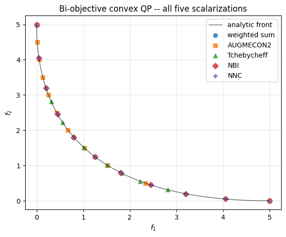
1.5 Compare all five methods#
fig, ax = plt.subplots(figsize=(6, 5))
ax.plot(ref_f1, ref_f2, "k-", lw=1, alpha=0.6, label="analytic front")
for name, front, marker in [
    ("weighted sum", front_ws, "o"),
    ("AUGMECON2", front_eps, "s"),
    ("Tchebycheff", front_tch, "^"),
    ("NBI", front_nbi, "D"),
    ("NNC", front_nnc, "P"),
]:
    obj = front.objectives()
    ax.scatter(obj[:, 0], obj[:, 1], marker=marker, label=name, alpha=0.8)
ax.set_xlabel("$f_1$")
ax.set_ylabel("$f_2$")
ax.set_title("Bi-objective convex QP -- all five scalarizations")
ax.legend()
ax.grid(alpha=0.3)
plt.tight_layout();
2. Hypervolume comparison#
The hypervolume indicator is the Lebesgue measure of the region dominated by a front with respect to a reference point (chosen beyond the nadir). It is Pareto-compliant – a front that dominates another has strictly larger hypervolume – so it is the standard scalar quality measure [Zitzler et al., 2000].
ref = np.array([5.5, 5.5])
rows = []
for name, f in [
    ("weighted_sum", front_ws),
    ("augmecon2", front_eps),
    ("tchebycheff", front_tch),
    ("nbi", front_nbi),
    ("nnc", front_nnc),
]:
    rows.append((name, f.n, f.hypervolume(reference=ref)))
for name, n, hv in rows:
    print(f"  {name:>14s}   n={n:3d}   hypervolume = {hv:.4f}")
    weighted_sum   n= 11   hypervolume = 25.1625
       augmecon2   n= 11   hypervolume = 24.5258
     tchebycheff   n= 11   hypervolume = 24.7531
             nbi   n= 11   hypervolume = 25.1625
             nnc   n= 11   hypervolume = 25.1625
3. A nonconvex front#
When the Pareto front is concave, the image set is not convex and weighted sum fails: for every \(w \ge 0\) the minimum is attained at an anchor, not in the front’s interior. AUGMECON2, Tchebycheff, NBI, and NNC all recover the full front.
The Pareto boundary is the quarter-arc of the unit circle, which is strictly concave.
def build_concave():
    m = dm.Model("concave")
    x = m.continuous("x", lb=0, ub=1)
    y = m.continuous("y", lb=0, ub=1)
    m.subject_to(x**2 + y**2 >= 1.0)
    return m, [x, y]


m, objs = build_concave()
c_ws = weighted_sum(m, objs, n_weights=11)
m, objs = build_concave()
c_tch = weighted_tchebycheff(m, objs, n_weights=11)
m, objs = build_concave()
c_eps = epsilon_constraint(m, objs, n_points=11)
m, objs = build_concave()
c_nbi = normal_boundary_intersection(m, objs, n_points=11)

fig, ax = plt.subplots(figsize=(6, 5))
theta = np.linspace(0, np.pi / 2, 201)
ax.plot(np.cos(theta), np.sin(theta), "k-", lw=1, alpha=0.6, label="true front")
for name, f, marker in [
    ("weighted sum", c_ws, "o"),
    ("AUGMECON2", c_eps, "s"),
    ("Tchebycheff", c_tch, "^"),
    ("NBI", c_nbi, "D"),
]:
    obj = f.objectives()
    ax.scatter(obj[:, 0], obj[:, 1], marker=marker, label=name, alpha=0.8)
ax.set_xlabel("$f_1$")
ax.set_ylabel("$f_2$")
ax.set_title("Concave Pareto front (weighted sum collapses to anchors)")
ax.legend()
ax.grid(alpha=0.3)
plt.tight_layout();

4. When to use which method#
Synthesis of the guidance in [Miettinen, 1999] and [Marler and Arora, 2004]:
Goal |
Method |
|---|---|
Convex front, simple baseline |
|
Guaranteed completeness on any front |
|
Nonconvex front, \(L_\infty\) semantics |
|
Uniform spacing, smooth convex front |
|
Robust geometric method with explicit normalization |
|
All methods share the same calling convention: pass the Model, the list
of objective Expression objects, optional senses=["min", ..., "max"],
and any solve_kwargs (e.g. time_limit=, gap_tolerance=). The
returned ParetoFront supports .summary(), .plot(),
.hypervolume(reference=...), and .filtered() (strict-nondominance
filter).
5. Side effects#
Scalarizers mutate the input Model: auxiliary parameters (and, for
AUGMECON, Tchebycheff, NBI, NNC, extra variables and constraints) are
added. The model’s original objective is restored on exit, but residual
auxiliary structure remains. If you intend to reuse the model for other
solves, build a fresh dm.Model each call. This matches the in-place
pattern used by discopt.ro.
6. Next steps#
For expensive objectives (each evaluation costs minutes or requires lab experiments) see the upcoming Bayesian multi-objective wrapper based on expected hypervolume improvement [Knowles, 2006].
For evolutionary multi-objective algorithms (NSGA-II, MOEA/D, NSGA-III) use
pymoo[Blank and Deb, 2020] to generate baseline fronts, then refine with adiscopt.moscalarization sweep.The full algorithmic background is in the
.crucible/wiki/methods/articles shipped with the repo.