Factor Screening with 2-Level Factorial Designs#
When you have a handful of candidate factors and the question is
“which ones actually matter?”, the right answer is rarely a
response-surface model — it’s a screening design. A two-level
full factorial probes every factor at a LOW and a HIGH setting,
in a structured way that gives orthogonal estimates of each main
effect at the smallest run count compatible with that goal
[Box et al., 2005].
When to use this notebook’s approach#
You have 2–7 candidate factors and want to filter the “vital few” before investing in a quadratic response-surface or mechanistic model.
Each factor has a sensible LOW and HIGH setting (continuous range endpoints, or two categorical levels you actually want to compare — catalyst A vs. B, supplier 1 vs. 2).
You can afford \(2^k\) runs (plus optional center points and replicates). For \(k = 3\) that’s 8 runs, for \(k = 5\) it’s 32. If you have more than ~7 factors, a half-fraction (resolution V) scales better; for now
discopt.doeonly supports full factorials.
Don’t use this template if you already know which factors matter and
want the optimum — switch to a response-surface design
(response-surface-2d / 3d) or to active-learning optimization
(see the active-learning.ipynb notebook). And don’t use it if your
factors are proportions of a blend summing to a constant — use the
Scheffé mixture templates instead.
Plan#
Build a \(2^3\) full factorial with three factors (one categorical), plus center points and a replicate.
Simulate a response with known true main effects and one interaction.
Compute signed effect estimates and visualize them on a Pareto chart.
Run an ANOVA to attach p-values and test whether the interactions are significant.
End with the CLI round trip and practical guidance.
import os
os.environ["JAX_PLATFORMS"] = "cpu"

import numpy as np
import matplotlib.pyplot as plt

from discopt.doe import (
    anova_report,
    effects_estimates,
    factorial_2level_design,
)

rng = np.random.default_rng(0)
1. Build the design#
Three factors with a deliberately mixed type signature:
temp— continuous, °C, LOW=80, HIGH=120catalyst— categorical, two suppliers A vs. Bpressure— continuous, bar, LOW=1, HIGH=5
We add 2 center-point runs per replicate so we can detect curvature, and 2 replicates so we have enough residual degrees of freedom for F-tests on interactions.
Heads up. Center points require all factors to be numeric, because the center is the midpoint. With a categorical factor in the mix,
factorial_2level_design(..., center_points=>0)will refuse — we’d have to encodecatalystas 0/1 first. Here we setcenter_points=0and instead usereplicates=2to get a residual df.
design = factorial_2level_design(
    factors={
        "temp":     (80.0, 120.0),
        "catalyst": ("A", "B"),
        "pressure": (1.0, 5.0),
    },
    center_points=0,
    replicates=2,
    seed=1,
)
print(f"{len(design.rows)} runs total (2^3 corners × 2 replicates = 16)")
print()
for r in design.rows[:8]:
    print(r)
print("...")
16 runs total (2^3 corners × 2 replicates = 16)

{'temp': 80.0, 'catalyst': 'B', 'pressure': 1.0, 'replicate': 0, 'is_center': False, 'run_order': 0}
{'temp': 80.0, 'catalyst': 'B', 'pressure': 1.0, 'replicate': 1, 'is_center': False, 'run_order': 1}
{'temp': 80.0, 'catalyst': 'A', 'pressure': 1.0, 'replicate': 0, 'is_center': False, 'run_order': 2}
{'temp': 120.0, 'catalyst': 'B', 'pressure': 1.0, 'replicate': 1, 'is_center': False, 'run_order': 3}
{'temp': 120.0, 'catalyst': 'B', 'pressure': 1.0, 'replicate': 0, 'is_center': False, 'run_order': 4}
{'temp': 120.0, 'catalyst': 'A', 'pressure': 5.0, 'replicate': 0, 'is_center': False, 'run_order': 5}
{'temp': 80.0, 'catalyst': 'B', 'pressure': 5.0, 'replicate': 0, 'is_center': False, 'run_order': 6}
{'temp': 80.0, 'catalyst': 'A', 'pressure': 1.0, 'replicate': 1, 'is_center': False, 'run_order': 7}
...
Two things to notice:
The
run_orderis randomized across the whole experiment, not per-replicate — that’s exactly the protection against time-trend nuisance factors that randomization is meant to give.The categorical factor
catalystshows up as'A'/'B'in the row dicts. The downstreameffects_estimatesandanova_reportfunctions both handle mixed numeric/string factor columns transparently.
2. Simulate responses#
We synthesize a response where temp and catalyst matter,
pressure does not, and there is a moderate temp × catalyst
interaction:
where each \(x\) is coded \(\pm 1\) for LOW / HIGH.
def code_factor(value, low, high):
    return -1.0 if value == low else +1.0

rng = np.random.default_rng(2)
rows_with_y = []
for r in design.rows:
    xt = code_factor(r["temp"], 80.0, 120.0)
    xc = code_factor(r["catalyst"], "A", "B")
    xp = code_factor(r["pressure"], 1.0, 5.0)
    y = 10.0 + 3.0 * xt + 2.0 * xc - 0.05 * xp + 1.5 * xt * xc + 0.5 * rng.normal()
    rows_with_y.append({**r, "y": float(y)})

for r in rows_with_y[:5]:
    print(r)
{'temp': 80.0, 'catalyst': 'B', 'pressure': 1.0, 'replicate': 0, 'is_center': False, 'run_order': 0, 'y': 7.644526690896767}
{'temp': 80.0, 'catalyst': 'B', 'pressure': 1.0, 'replicate': 1, 'is_center': False, 'run_order': 1, 'y': 7.288625779259627}
{'temp': 80.0, 'catalyst': 'A', 'pressure': 1.0, 'replicate': 0, 'is_center': False, 'run_order': 2, 'y': 6.343468228304053}
{'temp': 120.0, 'catalyst': 'B', 'pressure': 1.0, 'replicate': 1, 'is_center': False, 'run_order': 3, 'y': 15.329266308680072}
{'temp': 120.0, 'catalyst': 'B', 'pressure': 1.0, 'replicate': 0, 'is_center': False, 'run_order': 4, 'y': 17.449853691360453}
3. Signed main effects + a Pareto chart#
For a 2-level factorial the natural summary is the signed main effect for each factor:
effects_estimates returns this together with the standard error
and a t-statistic against the pooled residual, sorted by
\(|\text{effect}|\) descending. A Pareto chart of \(|\text{effect}|\)
is the standard visualization: it makes the few important factors
jump out from the rest.
effects = effects_estimates(rows_with_y, response="y")
for e in effects:
    print(
        f"  {e['factor']:10s}  effect = {e['effect']:+6.3f}   "
        f"se = {e['se']:.3f}   t = {e['t']:+6.2f}   "
        f"({e['low']!r} → {e['high']!r})"
    )
  temp        effect = +6.078   se = 1.369   t =  +4.44   (80.0 → 120.0)
  catalyst    effect = +3.936   se = 1.846   t =  +2.13   ('A' → 'B')
  pressure    effect = +0.020   se = 2.125   t =  +0.01   (1.0 → 5.0)
# Pareto chart of |effect|
labels = [e["factor"] for e in effects]
abs_eff = [abs(e["effect"]) for e in effects]
signs = ["+" if e["effect"] > 0 else "−" for e in effects]

# A rule-of-thumb significance reference: 2*se of the smallest factor's effect
ref = 2.0 * effects[-1]["se"] if effects[-1]["se"] > 0 else None

fig, ax = plt.subplots(figsize=(6, 3.5))
bars = ax.barh(labels[::-1], abs_eff[::-1],
               color=["C0" if s == "+" else "C3" for s in signs[::-1]])
for bar, s in zip(bars, signs[::-1]):
    ax.text(bar.get_width() + 0.05, bar.get_y() + bar.get_height()/2,
            s, va="center", fontsize=12, fontweight="bold")
if ref is not None:
    ax.axvline(ref, color="grey", linestyle="--", alpha=0.6,
               label=f"2·SE ≈ {ref:.2f}")
    ax.legend()
ax.set_xlabel("|effect estimate|")
ax.set_title("Pareto chart of main effects")
plt.tight_layout(); plt.show()
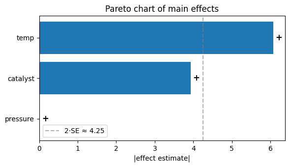
Reading the chart. Bars above the dashed 2·SE line are
plausibly real effects; bars below it are probably noise. In our
synthesized data temp (effect ≈ +6) and catalyst (effect ≈ +4)
clear the bar comfortably; pressure (effect ≈ −0.1) does not.
The sign in the right margin tells you whether HIGH increases or
decreases the response.
Note that the signed effects are scaled by a factor of 2 relative to
the regression coefficients (because the corners are at \(\pm 1\)
rather than 0 vs 1) — so effect = +6 corresponds to the true
coefficient \(b = +3\) from our simulation.
4. ANOVA — including the interaction test#
The Pareto chart is great for ranking, but it does not test the
no-interaction assumption. anova_report does that. By passing
interactions=[("temp", "catalyst"), ("temp", "pressure"), …] we
ask for a Type-I sum-of-squares decomposition that splits out each
interaction’s variance and gives it an F + p value.
table = anova_report(
    rows_with_y,
    response="y",
    factors=["temp", "catalyst", "pressure"],
    interactions=[
        ("temp", "catalyst"),
        ("temp", "pressure"),
        ("catalyst", "pressure"),
    ],
)
print(table.summary())
Source                         SS    df           MS         F          p
-------------------------------------------------------------------------
temp                     147.7708     1     147.7708   424.041  7.018e-09
catalyst                  61.9663     1      61.9663   177.818  3.121e-07
pressure                   0.0016     1       0.0016     0.005     0.9477
temp:catalyst             39.7075     1      39.7075   113.944  2.073e-06
temp:pressure              0.1852     1       0.1852     0.531     0.4846
catalyst:pressure          0.0098     1       0.0098     0.028     0.8706
Residual                   3.1363     9       0.3485       ---        ---
Total                    252.7775    15       0.0000       ---        ---
As expected:
tempandcatalystare highly significant — tiny p-values.pressureis non-significant — its p-value is large, so we can drop it from any downstream model.temp × catalystis significant — confirming the interaction we baked into the simulation. The other interactions are noise.
This is the screening conclusion: keep temp and catalyst (and
their interaction); drop pressure. Now go run a focused
response-surface or active-learning optimization on the surviving
factors.
5. Fractional factorials for many factors#
A full \(2^k\) factorial doubles in size with every factor you add. For \(k = 6\) that’s 64 runs even before replication; for \(k = 8\) it is 256. A fractional factorial picks \(2^{k-p}\) of the corners so that:
every main effect remains estimable, and
the kept effect columns are pairwise orthogonal at the requested resolution.
Resolution III keeps main effects clear of one another; IV also
keeps them clear of two-factor interactions; V additionally keeps
every two-factor interaction clear of the others. The classical
construction picks defining contrasts by hand; discopt.doe
formulates the row selection as a small MILP and lets the solver
choose them.
Below we generate a resolution-IV half-fraction of a \(2^5\) design (16 runs instead of 32) and verify the orthogonality structure by inspecting the Gram matrix of the model columns.
import itertools

from discopt.doe import fractional_factorial_design

frac = fractional_factorial_design(
    factors={f: (-1.0, 1.0) for f in ["A", "B", "C", "D", "E"]},
    n_runs=16,
    resolution=4,
    seed=0,
)
print(f"{len(frac.rows)} runs (half-fraction of 2^5 = 32)")

# Code the design as a ±1 matrix.
M = np.array([[r[f] for f in frac.factors] for r in frac.rows], dtype=int)

# Mains are balanced and pairwise orthogonal — diagonal Gram.
print("\nmain-effect Gram matrix (off-diagonal zeros ⇒ orthogonal):")
print(M.T @ M)

# Every 3-factor interaction column is balanced ⇒ no main is aliased
# with any 2FI (the defining property of resolution IV).
imbalances = [
    abs((M[:, i] * M[:, j] * M[:, k]).sum())
    for i, j, k in itertools.combinations(range(5), 3)
]
print(f"\nmax |Σ 3FI column| across all triples: {max(imbalances)} "
      f"(0 ⇒ main effects clear of every 2FI)")
16 runs (half-fraction of 2^5 = 32)

main-effect Gram matrix (off-diagonal zeros ⇒ orthogonal):
[[16  0  0  0  0]
 [ 0 16  0  0  0]
 [ 0  0 16  0  0]
 [ 0  0  0 16  0]
 [ 0  0  0  0 16]]

max |Σ 3FI column| across all triples: 0 (0 ⇒ main effects clear of every 2FI)
Sixteen runs cover the five factors and let us fit all five main
effects without any aliasing into the two-factor interactions —
the kind of return on investment fractional designs are built for.
Switch the call to resolution=5 and you get the classical 16-run
\(2^{5-1}_V\) design with every two-factor interaction also clear.
6. CLI round trip#
The whole workflow is also available from the command line. The workbook stores categorical factor values as strings, so it round-trips through Excel without quoting headaches.
discopt doe new factorial-2level \
    --factor "temp:80:120" \
    --factor "catalyst:A:B" \
    --factor "pressure:1:5" \
    --replicates 2 \
    --out screen.xlsx

# … run the experiments, fill in the y column …

discopt doe anova screen.xlsx \
    --interaction "temp:catalyst" \
    --interaction "temp:pressure" \
    --interaction "catalyst:pressure"
For purely numeric factors you can also add --center-points 2 to
the new step to enable a curvature test.
7. Practical guidance#
Run-count guide#
\(k\) |
\(2^k\) runs |
With 2 replicates |
With 2 center points/rep |
|---|---|---|---|
3 |
8 |
16 |
20 |
4 |
16 |
32 |
36 |
5 |
32 |
64 |
68 |
6 |
64 |
128 |
132 |
7 |
128 |
256 |
260 |
Beyond \(k = 7\) a fractional factorial cuts the run count to \(2^{k-p}\) corners while still letting you estimate every main effect — see Section 5 below for a MILP-based generator. For even larger \(k\), a Plackett-Burman [] design covers \(k\) factors in \(k+1\) runs at resolution III (not yet implemented here).
When to add center points#
Center points serve two purposes — a curvature test and a pure-error variance estimate. They require all factors to be numeric, so encode categoricals as 0/1 first if you need them.
When the screening tells you to keep more factors#
If 3 or fewer factors survive screening, jump to a
response-surface-2d/3ddesign or tooptimize_round(active learning).If more than 4 survive, consider a second screening round on the survivors at narrower bounds before optimizing — the response often becomes more nonlinear near the optimum.
Avoid this template if…#
…the runs of your experiment are stratified (operator, batch, day) and the strata can interact with the factors. Use a Latin square or factorial-with-block design and check
latin-designs.ipynb.…your factors are blend proportions; use Scheffé mixture designs.
References#
Box et al. [2005] — the standard practitioner reference on screening and response-surface methodology.
— comprehensive textbook treatment of factorial designs, replication, and ANOVA.
— fractional designs for screening many factors in few runs.