Active-Learning Optimization with a Surrogate#
This notebook walks through discopt.doe.optimize_round — an
active-learning loop that finds the input minimizing or maximizing
a measured response, using as few experiments as possible.
The idea, going back at least to Box and Wilson [1951] for response-surface methods and Jones et al. [1998] for Bayesian optimization with Gaussian processes, is to never run a fixed design. Instead, after every batch of experiments:
fit a probabilistic surrogate model to the responses you have so far;
use an acquisition function to score where the next experiment would be most useful — exploiting the surrogate’s predicted optimum, while exploring where the surrogate is uncertain;
run the recommended batch, append the results, and repeat.
The key abstraction is that the optimizer only ever needs the surrogate’s predicted mean and standard deviation at candidate points. Anything that can produce those two arrays — a GP with a kernel of your choice [Rasmussen and Williams, 2006], a Bayesian linear model, an LPR local-prediction regressor, your own object — slots in.
When to use this notebook’s approach#
You want the best input, not the most precise model parameters. (For parameter estimation, use
optimal_experimentinstead.)Experiments are expensive — full factorials or response-surface designs are too wasteful.
You can usually already screen out irrelevant factors with
factorial_2level_designbefore optimizing.
Plan of this notebook#
A 1D toy problem with closed-form ground truth, to build intuition for the loop.
The same problem with a user-supplied GP kernel (Matern + white noise), to demonstrate the bring-your-own-model path.
A 2D example showing batch recommendation + the GP’s posterior.
Practical guidance: choosing a surrogate, choosing an acquisition, stopping criteria, and known limitations.
import os
os.environ["JAX_PLATFORMS"] = "cpu"

import warnings
import numpy as np
import matplotlib.pyplot as plt
from openpyxl import load_workbook

from discopt.doe import (
    OptimizationCriterion,
    optimize_round,
)
from discopt.doe.workbook import InputSpec, Workbook

warnings.filterwarnings("ignore", message=".*ConvergenceWarning.*")
rng = np.random.default_rng(0)
1. A 1D problem with a true optimum#
The simulated response is
so the true maximum is \(y^\star = 3\) at \(x^\star = 2\). The optimizer does not know this — it only sees the responses we feed it through the workbook.
We start the loop by seeding it with four random runs.
def truth_1d(x):
    return -(x - 2.0) ** 2 + 3.0 + 0.05 * np.random.default_rng().normal()

WORKBOOK = "/tmp/active_learning_1d.xlsx"
Workbook.create(
    WORKBOOK,
    template=None,
    template_args={},
    input_specs=[InputSpec("x", -5.0, 5.0)],
    criterion="custom",
    measurement_error=0.05,
    seed=0,
    response_name="y",
)
wb = Workbook.open(WORKBOOK)
init_x = np.array([-4.0, -1.0, 1.5, 4.0])
wb.append_runs(0, [{"x": float(x)} for x in init_x])
wb.save()

# Fill the responses we "measured"
book = load_workbook(WORKBOOK)
sh = book["runs"]
for i, x in enumerate(init_x, start=2):
    sh.cell(row=i, column=4, value=float(truth_1d(x)))
book.save(WORKBOOK)

list(Workbook.open(WORKBOOK).completed_runs())
[{'run_id': 1,
  'batch': 0,
  'x': -4,
  'y': -33.02803072022783,
  'measured_at': None},
 {'run_id': 2,
  'batch': 0,
  'x': -1,
  'y': -5.988287940936011,
  'measured_at': None},
 {'run_id': 3,
  'batch': 0,
  'x': 1.5,
  'y': 2.646758018093148,
  'measured_at': None},
 {'run_id': 4,
  'batch': 0,
  'x': 4,
  'y': -0.9620965067672387,
  'measured_at': None}]
Running one round#
A single call to optimize_round does the four steps in turn —
read completed runs → fit the surrogate → score candidates → append
the next batch.
def fill_responses(path, run_ids, designs, truth_fn):
    book = load_workbook(path)
    sh = book["runs"]
    by_id = {rid: d for rid, d in zip(run_ids, designs)}
    for row in sh.iter_rows(min_row=2):
        rid = row[0].value
        if rid in by_id:
            row[3].value = float(truth_fn(by_id[rid]["x"]))
    book.save(path)


result = optimize_round(
    workbook=WORKBOOK,
    criterion=OptimizationCriterion.MAXIMIZE,
    surrogate="gp",                        # string preset
    acquisition="expected_improvement",    # the standard BO choice
    batch_size=2,
    seed=0,
)
print("next batch:", result.next_designs)
print("incumbent so far:", result.incumbent_x, "->", round(result.incumbent_y, 3))
fill_responses(WORKBOOK, result.new_run_ids, result.next_designs, truth_1d)
next batch: [{'x': 2.4120481312274933}, {'x': 1.1990866344422102}]
incumbent so far: {'x': 1.5} -> 2.647
/Users/jkitchin/Dropbox/uv/.venv/lib/python3.12/site-packages/sklearn/gaussian_process/kernels.py:442: ConvergenceWarning: The optimal value found for dimension 0 of parameter k2__noise_level is close to the specified lower bound 1e-08. Decreasing the bound and calling fit again may find a better value.
  warnings.warn(
Iterating to convergence#
We run six rounds of two experiments each and watch the incumbent approach the truth.
history = []
for rnd in range(6):
    result = optimize_round(
        workbook=WORKBOOK,
        criterion=OptimizationCriterion.MAXIMIZE,
        surrogate="gp",
        acquisition="expected_improvement",
        batch_size=2,
        seed=rnd + 1,
    )
    fill_responses(WORKBOOK, result.new_run_ids, result.next_designs, truth_1d)
    completed = Workbook.open(WORKBOOK).completed_runs()
    ys = [float(r["y"]) for r in completed]
    best = max(range(len(ys)), key=lambda i: ys[i])
    history.append({
        "round": rnd,
        "n_runs": len(completed),
        "best_y": ys[best],
        "best_x": float(completed[best]["x"]),
    })

for h in history:
    print(h)
print()
print(f"truth max: y=3.0 at x=2.0")
/Users/jkitchin/Dropbox/uv/.venv/lib/python3.12/site-packages/sklearn/gaussian_process/kernels.py:442: ConvergenceWarning: The optimal value found for dimension 0 of parameter k2__noise_level is close to the specified lower bound 1e-08. Decreasing the bound and calling fit again may find a better value.
  warnings.warn(
/Users/jkitchin/Dropbox/uv/.venv/lib/python3.12/site-packages/sklearn/gaussian_process/_gpr.py:660: ConvergenceWarning: lbfgs failed to converge (status=2):
ABNORMAL: .

Increase the number of iterations (max_iter) or scale the data as shown in:
    https://scikit-learn.org/stable/modules/preprocessing.html
  _check_optimize_result("lbfgs", opt_res)
{'round': 0, 'n_runs': 8, 'best_y': 3.125594830793453, 'best_x': 2.136436272412539}
{'round': 1, 'n_runs': 10, 'best_y': 3.125594830793453, 'best_x': 2.136436272412539}
{'round': 2, 'n_runs': 12, 'best_y': 3.125594830793453, 'best_x': 2.136436272412539}
{'round': 3, 'n_runs': 14, 'best_y': 3.125594830793453, 'best_x': 2.136436272412539}
{'round': 4, 'n_runs': 16, 'best_y': 3.125594830793453, 'best_x': 2.136436272412539}
{'round': 5, 'n_runs': 18, 'best_y': 3.125594830793453, 'best_x': 2.136436272412539}

truth max: y=3.0 at x=2.0
Visualizing what the surrogate believes#
After all rounds we refit the GP to every completed run and plot its mean + 95% credible band, the truth, and the points the optimizer chose to evaluate.
from discopt.doe.surrogate import coerce_surrogate

completed = Workbook.open(WORKBOOK).completed_runs()
X = np.array([[float(r["x"])] for r in completed])
y = np.array([float(r["y"]) for r in completed])

s = coerce_surrogate("gp")
s.fit(X, y)

xs = np.linspace(-5, 5, 400).reshape(-1, 1)
mu, sd = s.predict(xs)

fig, ax = plt.subplots(figsize=(7, 4))
ax.plot(xs.ravel(), -(xs.ravel() - 2.0) ** 2 + 3.0, "k--", label="truth")
ax.plot(xs.ravel(), mu, "C0-", label="GP mean")
ax.fill_between(xs.ravel(), mu - 1.96 * sd, mu + 1.96 * sd,
                color="C0", alpha=0.2, label="GP 95%")
ax.scatter(X[: len(init_x), 0], y[: len(init_x)], color="k",
           marker="o", label="seed runs")
ax.scatter(X[len(init_x):, 0], y[len(init_x):], color="C3",
           marker="x", label="active-learning picks")
ax.axvline(2.0, color="grey", linestyle=":", alpha=0.4)
ax.set_xlabel("x"); ax.set_ylabel("y")
ax.set_title("GP surrogate after the loop")
ax.legend(loc="lower center")
plt.tight_layout(); plt.show()
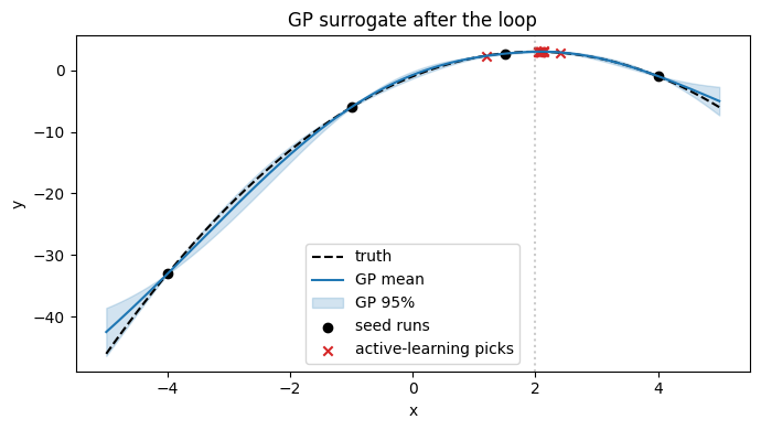
The picks cluster near \(x = 2\) — exactly where they should — but notice a few exploration picks well away from the incumbent. That is the EI acquisition doing its job: it discounts the predicted-mean gain by the surrogate’s uncertainty, so points where the GP is nervous still get sampled.
2. Bring-your-own GP kernel#
The string preset "gp" chooses Matern(5/2) + white noise. If you
want a different kernel — or any other UQ-providing scikit-learn
estimator — pass the estimator directly. The adapter detects
predict(X, return_std=True) and wires it up automatically.
from sklearn.gaussian_process import GaussianProcessRegressor
from sklearn.gaussian_process.kernels import RBF, ConstantKernel, WhiteKernel

# Reset workbook to compare apples to apples
WORKBOOK2 = "/tmp/active_learning_1d_rbf.xlsx"
Workbook.create(
    WORKBOOK2, template=None, template_args={},
    input_specs=[InputSpec("x", -5.0, 5.0)],
    criterion="custom", measurement_error=0.05, seed=0, response_name="y",
)
wb2 = Workbook.open(WORKBOOK2)
wb2.append_runs(0, [{"x": float(x)} for x in init_x])
wb2.save()
book = load_workbook(WORKBOOK2)
sh = book["runs"]
for i, x in enumerate(init_x, start=2):
    sh.cell(row=i, column=4, value=float(truth_1d(x)))
book.save(WORKBOOK2)

my_gp = GaussianProcessRegressor(
    kernel=ConstantKernel(1.0) * RBF(length_scale=1.0)
           + WhiteKernel(noise_level=0.01),
    normalize_y=True,
    n_restarts_optimizer=4,
)

for rnd in range(4):
    result = optimize_round(
        workbook=WORKBOOK2,
        criterion=OptimizationCriterion.MAXIMIZE,
        surrogate=my_gp,                  # <-- the estimator directly
        acquisition="expected_improvement",
        batch_size=2,
        seed=rnd + 100,
    )
    fill_responses(WORKBOOK2, result.new_run_ids, result.next_designs, truth_1d)

completed = Workbook.open(WORKBOOK2).completed_runs()
ys = [float(r["y"]) for r in completed]
best = max(range(len(ys)), key=lambda i: ys[i])
print(f"RBF kernel: best y = {ys[best]:.3f} at x = {float(completed[best]['x']):.3f}")
print(f"using {len(completed)} total runs")
/Users/jkitchin/Dropbox/uv/.venv/lib/python3.12/site-packages/sklearn/gaussian_process/kernels.py:442: ConvergenceWarning: The optimal value found for dimension 0 of parameter k2__noise_level is close to the specified lower bound 1e-05. Decreasing the bound and calling fit again may find a better value.
  warnings.warn(
RBF kernel: best y = 3.073 at x = 1.934
using 12 total runs
The same code path also accepts other UQ models. For example
pycse.sklearn.lpr.LinearLPR exposes predict(X, return_interval=True);
the adapter detects that and converts the interval to a pseudo-σ
without any wrapper code on your side. If you have your own
Bayesian model, implement the two-method Surrogate protocol and
set _is_discopt_surrogate = True on the class to bypass the
adapter entirely.
3. A 2D example#
Two inputs, a banana-ish response, four random seed points, six rounds of three picks each. The plot shows where the optimizer chose to evaluate, overlaid on the GP’s posterior mean.
def truth_2d(x1, x2):
    return -((x1 - 1.0) ** 2 + 4 * (x2 - 0.5 * x1 ** 2) ** 2) + 0.02 * np.random.default_rng().normal()

WORKBOOK3 = "/tmp/active_learning_2d.xlsx"
Workbook.create(
    WORKBOOK3, template=None, template_args={},
    input_specs=[InputSpec("x1", -2.0, 2.0), InputSpec("x2", -2.0, 2.0)],
    criterion="custom", measurement_error=0.05, seed=0, response_name="y",
)
wb3 = Workbook.open(WORKBOOK3)
seed_pts = rng.uniform(-2, 2, size=(6, 2))
wb3.append_runs(0, [{"x1": float(p[0]), "x2": float(p[1])} for p in seed_pts])
wb3.save()
book = load_workbook(WORKBOOK3)
sh = book["runs"]
for i, p in enumerate(seed_pts, start=2):
    sh.cell(row=i, column=5, value=float(truth_2d(p[0], p[1])))
book.save(WORKBOOK3)

def fill_2d(path, run_ids, designs, truth_fn):
    book = load_workbook(path)
    sh = book["runs"]
    by_id = {rid: d for rid, d in zip(run_ids, designs)}
    for row in sh.iter_rows(min_row=2):
        rid = row[0].value
        if rid in by_id:
            d = by_id[rid]
            row[4].value = float(truth_fn(d["x1"], d["x2"]))
    book.save(path)

for rnd in range(6):
    result = optimize_round(
        workbook=WORKBOOK3,
        criterion=OptimizationCriterion.MAXIMIZE,
        surrogate="gp",
        acquisition="expected_improvement",
        batch_size=3,
        seed=rnd,
    )
    fill_2d(WORKBOOK3, result.new_run_ids, result.next_designs, truth_2d)

completed = Workbook.open(WORKBOOK3).completed_runs()
X = np.array([[float(r["x1"]), float(r["x2"])] for r in completed])
y = np.array([float(r["y"]) for r in completed])
print(f"2D run: {len(completed)} total runs, best y={y.max():.3f} at {X[y.argmax()]}")
print(f"truth max: y=0 at (x1, x2) = (1, 0.5)")
/Users/jkitchin/Dropbox/uv/.venv/lib/python3.12/site-packages/sklearn/gaussian_process/kernels.py:442: ConvergenceWarning: The optimal value found for dimension 0 of parameter k2__noise_level is close to the specified lower bound 1e-08. Decreasing the bound and calling fit again may find a better value.
  warnings.warn(
/Users/jkitchin/Dropbox/uv/.venv/lib/python3.12/site-packages/sklearn/gaussian_process/_gpr.py:660: ConvergenceWarning: lbfgs failed to converge (status=2):
ABNORMAL: .

Increase the number of iterations (max_iter) or scale the data as shown in:
    https://scikit-learn.org/stable/modules/preprocessing.html
  _check_optimize_result("lbfgs", opt_res)
2D run: 24 total runs, best y=0.031 at [1.06848741 0.54139654]
truth max: y=0 at (x1, x2) = (1, 0.5)
# Visualize: GP posterior mean + sampled points
from discopt.doe.surrogate import coerce_surrogate

s = coerce_surrogate("gp")
s.fit(X, y)

g = np.linspace(-2, 2, 80)
G1, G2 = np.meshgrid(g, g)
Xg = np.column_stack([G1.ravel(), G2.ravel()])
mu, _ = s.predict(Xg)
Mu = mu.reshape(G1.shape)

fig, ax = plt.subplots(figsize=(6, 5))
cs = ax.contourf(G1, G2, Mu, levels=20, cmap="viridis")
plt.colorbar(cs, ax=ax, label="GP mean")
ax.scatter(X[:6, 0], X[:6, 1], color="white", edgecolor="k",
           marker="o", s=60, label="seed")
ax.scatter(X[6:, 0], X[6:, 1], color="red", edgecolor="k",
           marker="x", s=60, label="active-learning")
ax.scatter([1.0], [0.5], color="yellow", marker="*", s=200,
           edgecolor="k", label="true max")
ax.set_xlabel("x1"); ax.set_ylabel("x2"); ax.legend(loc="lower left")
ax.set_title("GP posterior mean + active-learning picks")
plt.tight_layout(); plt.show()
/var/folders/gq/k1kgbl7n539_4dl1md8x3jt80000gn/T/ipykernel_99858/2070178741.py:18: UserWarning: You passed a edgecolor/edgecolors ('k') for an unfilled marker ('x').  Matplotlib is ignoring the edgecolor in favor of the facecolor.  This behavior may change in the future.
  ax.scatter(X[6:, 0], X[6:, 1], color="red", edgecolor="k",

4. Practical guidance#
Choosing a surrogate#
Surrogate |
When |
Tradeoff |
|---|---|---|
|
default; few runs (< 200); smooth response |
scales as \(O(n^3)\); needs hyperparameter fit |
|
classical Box-Wilson; want interpretable model |
restricted to degree-2; weak far from sampled X |
|
you want a specific kernel |
same scaling as |
|
LPR’s local linear UQ |
adapter converts interval to σ automatically |
Custom |
you have a bespoke Bayesian model |
full control; you implement |
Choosing an acquisition#
expected_improvement— start here. Self-tuning balance of exploration and exploitation. The default in Jones et al. [1998].ucb/lcb— same idea, simpler math; tune viaacquisition_kwargs={"kappa": ...}. Larger κ → more exploration.steepest_ascent— Box-Wilson behavior; ignores uncertainty. Pair with"response-surface"if you want to reproduce classical RSM. Don’t pair with a GP — you’d be throwing away the σ.
Stopping#
There is no fixed budget. Common heuristics:
stop when the incumbent has not improved for \(k\) rounds;
stop when the acquisition score at the best candidate falls below a tolerance (low EI means the GP no longer expects improvement anywhere);
stop when you’ve spent the budget you can afford.
Limitations of the current implementation#
Inputs must be numeric in the workbook. Encode categorical factors as 0/1 indicators upstream.
Constraints other than the input box bounds are not yet supported.
The greedy mean-imputation batch construction is fast but suboptimal for very large batches; for \(\text{batch} > 8\) consider running rounds with smaller batches more often.
References#
Box and Wilson [1951] — classical steepest-ascent / response-surface methodology.
Jones et al. [1998] — Efficient Global Optimization (EGO): Kriging surrogate + Expected Improvement.
Rasmussen and Williams [2006] — the standard reference on GP regression.
Snoek et al. [2012] — modern recipes for batch Bayesian optimization in hyperparameter tuning, applicable to physical experimentation as well.