Model-Based Active Learning for Response Optimization#
The active-learning.ipynb notebook used a black-box surrogate
(a Gaussian process) to drive Bayesian optimization. The GP learns
the response shape entirely from data and knows nothing about the
underlying physics. That’s a fine default when you have no model in
hand — but if you do have one (a kinetic rate law, an isotherm,
a transport correlation), you can do much better with the same
acquisition machinery.
This notebook walks through
:func:discopt.doe.model_based_optimize_round, which uses a
mechanistic / parametric model as the surrogate. The same
:class:~discopt.estimate.Experiment interface used by
:func:~discopt.doe.estimate_parameters and
:func:~discopt.doe.optimal_experiment plugs straight in.
When to use this notebook’s approach#
You have a parametric model
y = f(d; θ)you trust the form of, with unknown parameters θ you’d like to estimate as you go.Experiments are expensive: 3-10 runs total, not 30+.
You may want to extrapolate outside the sampled region (a GP cannot do this credibly; a correct mechanistic model can).
Your factors may be discrete / categorical and a GP would be awkward; the mechanistic model handles them natively.
Don’t use this when you don’t trust the functional form — a wrong model gives confidently wrong recommendations. The empirical GP path is safer there. See [Franceschini and Macchietto, 2008] for a survey of the tradeoffs.
Plan#
Set up a toy problem with a known mechanistic model (a saturating Michaelis-Menten-style response).
Generate a tiny seed dataset (4 runs).
Run one round of
model_based_optimize_round— it refits the parameters and recommends the next batch.Iterate to convergence; compare run-count to the GP version on the same problem.
Show the parameter trajectory — the optimization byproduct is a calibrated model.
import os
os.environ["JAX_PLATFORMS"] = "cpu"

import warnings
warnings.filterwarnings("ignore", category=UserWarning)

import numpy as np
import matplotlib.pyplot as plt

import discopt.modeling as dm
from discopt.estimate import Experiment, ExperimentModel
from discopt.doe import (
    OptimizationCriterion,
    model_based_optimize_round,
    optimize_round,
)
from discopt.doe.workbook import InputSpec, Workbook

rng = np.random.default_rng(0)
1. A mechanistic toy problem#
Imagine optimizing the substrate concentration \(S\) in an enzymatic reactor to maximize the volumetric product rate. The mechanism is saturating in \(S\) but the enzyme is inhibited at very high \(S\):
We have three unknown parameters \(\theta = (V_\text{max}, K_m, \alpha)\). The “truth” used to simulate experiments is
That gives a maximum near \(S \approx 3.6\) with \(y^{\star} \approx 1.6\), sitting well outside a span you’d cover with 3-4 corner points. A GP that has not been told this is the shape will not extrapolate to find that maximum from 3-4 corners; the mechanistic model will.
def truth(S, noise_sd=0.02, rng=rng):
    y = 2.0 * S / (0.5 + S) * np.exp(-0.05 * S)
    return float(y + noise_sd * rng.normal())


# Plot the true response surface
S_grid = np.linspace(0.05, 10.0, 200)
y_true = 2.0 * S_grid / (0.5 + S_grid) * np.exp(-0.05 * S_grid)

plt.figure(figsize=(5, 3))
plt.plot(S_grid, y_true, "k-", label="truth")
S_argmax = S_grid[np.argmax(y_true)]
plt.axvline(S_argmax, ls="--", color="grey",
            label=f"argmax ≈ {S_argmax:.2f}")
plt.xlabel("S")
plt.ylabel("y")
plt.title("True (hidden) response y(S)")
plt.legend()
plt.tight_layout(); plt.show()

2. Express the model as a discopt Experiment#
The Experiment class is the same one used by
discopt.estimate.estimate_parameters and
discopt.doe.optimal_experiment. You implement create_model(**kwargs),
returning an ExperimentModel that names the unknown parameters, the
design inputs, the predicted responses, and the measurement noise.
class MichaelisMentenWithInhibition(Experiment):
    def create_model(self, Vmax=1.0, Km=1.0, alpha=0.0):
        m = dm.Model("mm_inh")
        Vmax_var = m.continuous("Vmax", lb=0.01, ub=10.0)
        Km_var = m.continuous("Km", lb=0.01, ub=10.0)
        alpha_var = m.continuous("alpha", lb=0.0, ub=1.0)
        S = m.continuous("S", lb=0.05, ub=10.0)

        # discopt.modeling has exp/log via the dm namespace
        y_expr = Vmax_var * S / (Km_var + S) * dm.exp(-alpha_var * S)

        return ExperimentModel(
            model=m,
            unknown_parameters={"Vmax": Vmax_var, "Km": Km_var, "alpha": alpha_var},
            design_inputs={"S": S},
            responses={"y": y_expr},
            measurement_error={"y": 0.02},
        )


exp = MichaelisMentenWithInhibition()
print(f"unknown_parameters: {list(exp.create_model().unknown_parameters)}")
print(f"design_inputs: {list(exp.create_model().design_inputs)}")
unknown_parameters: ['Vmax', 'Km', 'alpha']
design_inputs: ['S']
3. Build a tiny seed workbook#
Active learning needs some data to fit parameters from. We seed with 4 well-spread points covering the design range. Realistically the seed is the cheapest exploratory data you have on hand.
tmp_path = "model_based_demo.xlsx"
Workbook.create(
    tmp_path,
    template=None,
    template_args={},
    input_specs=[InputSpec("S", 0.05, 10.0)],
    criterion="model-based",
    measurement_error=0.02,
    seed=0,
    response_name="y",
    module_callable=None,
    param_initial_guess={"Vmax": 1.0, "Km": 1.0, "alpha": 0.0},
)
wb = Workbook.open(tmp_path)
seed_xs = np.array([0.5, 2.5, 5.0, 9.0])
wb.append_runs(0, [{"S": float(s)} for s in seed_xs])
wb.save()

# Fill in the response column
from openpyxl import load_workbook
book = load_workbook(tmp_path)
sh = book["runs"]
for i, s in enumerate(seed_xs, start=2):
    sh.cell(row=i, column=4, value=truth(s, rng=np.random.default_rng(int(s * 100))))
book.save(tmp_path)

# Show what's in the workbook
for r in Workbook.open(tmp_path).completed_runs():
    print(f"S = {r['S']:5.2f}  →  y = {r['y']:.3f}")
S =  0.50  →  y = 0.985
S =  2.50  →  y = 1.453
S =  5.00  →  y = 1.430
S =  9.00  →  y = 1.207
4. One round of model-based active learning#
model_based_optimize_round does the following inside the box:
Reads the completed runs from the workbook.
Fits \(\theta = (V_\text{max}, K_m, \alpha)\) by maximum likelihood (Gauss-Newton with JAX-computed Jacobians).
Computes the parameter covariance \(\Sigma_\theta \approx \mathrm{FIM}^{-1}\) at the fit.
Samples a Sobol cloud of candidate \(S\) values.
For each candidate, predicts response mean \(\mu(S) = f(S; \hat\theta)\) and std via linearization, \(\sigma^2(S) \approx \nabla_\theta f \cdot \Sigma_\theta \cdot \nabla_\theta f^\top + \sigma_\text{meas}^2\).
Scores candidates with the chosen acquisition (expected improvement here).
Picks the top \(K\) for the next batch using a fantasy-mean refit to diversify the batch.
We need only the workbook — the Experiment will be rebuilt from its metadata (if a built-in template) or you can pass it explicitly (as we do here, because we use a custom Experiment).
result = model_based_optimize_round(
    workbook=tmp_path,
    experiment=exp,
    initial_guess={"Vmax": 1.0, "Km": 1.0, "alpha": 0.0},
    criterion=OptimizationCriterion.MAXIMIZE,
    acquisition="expected_improvement",
    batch_size=2,
    seed=0,
)

print("Fitted parameters:")
for name, value in result.parameters.items():
    se = result.parameter_se[name]
    print(f"  {name:6s} = {value:8.4f}  ± {se:.4f}")
print()
print(f"Incumbent so far: y = {result.incumbent_y:.4f} at S = {result.incumbent_x['S']:.3f}")
print(f"Next batch: {[d['S'] for d in result.next_designs]}")
print(f"log10 det FIM = {result.fim_log_det / np.log(10):.2f}")
Fitted parameters:
  Vmax   =   1.9664  ± 0.0479
  Km     =   0.4770  ± 0.0366
  alpha  =   0.0479  ± 0.0036

Incumbent so far: y = 1.4529 at S = 2.500
Next batch: [2.918644094793126, 2.9227032253053036]
log10 det FIM = 11.90
Two observations:
The parameters are estimated and their uncertainty is reported. The standard errors tell you which parameter the next experiment will tighten the most.
The recommended next batch lives near the model’s predicted maximum — because that’s where EI is largest — but the uncertainty also pulls the second point of the batch toward a diverse location.
5. Closing the loop#
def fill_responses(path, run_ids, designs, truth_fn):
    book = load_workbook(path)
    sh = book["runs"]
    by_id = {rid: d for rid, d in zip(run_ids, designs)}
    for row in sh.iter_rows(min_row=2):
        rid = row[0].value
        if rid in by_id:
            row[3].value = truth_fn(by_id[rid]["S"])
    book.save(path)


# Carry forward the design we just got
fill_responses(tmp_path, result.new_run_ids, result.next_designs,
               lambda s: truth(s, rng=np.random.default_rng(int(s * 1000) + 11)))

history = [{"n": len(seed_xs),
            "best_y": max(float(r["y"]) for r in Workbook.open(tmp_path).completed_runs())}]

for rnd in range(4):
    result = model_based_optimize_round(
        workbook=tmp_path,
        experiment=exp,
        initial_guess=result.parameters,    # warm-start from previous fit
        criterion=OptimizationCriterion.MAXIMIZE,
        acquisition="expected_improvement",
        batch_size=2,
        seed=rnd + 1,
    )
    fill_responses(tmp_path, result.new_run_ids, result.next_designs,
                   lambda s: truth(s, rng=np.random.default_rng(int(s * 1000) + rnd * 31)))
    completed = Workbook.open(tmp_path).completed_runs()
    history.append({"n": len(completed),
                    "best_y": max(float(r["y"]) for r in completed)})

print("Best-so-far trajectory:")
for h in history:
    print(f"  n = {h['n']:3d}  best y = {h['best_y']:.4f}")
Best-so-far trajectory:
  n =   4  best y = 1.5113
  n =   8  best y = 1.5113
  n =  10  best y = 1.5113
  n =  12  best y = 1.5113
  n =  14  best y = 1.5113
# Visualize convergence: model-based with very few runs
completed = Workbook.open(tmp_path).completed_runs()
S_obs = np.array([r["S"] for r in completed])
y_obs = np.array([r["y"] for r in completed])

# Refit a final surrogate to show the calibrated mean prediction
from discopt.doe.model_based import ParametricSurrogate
final = ParametricSurrogate(
    exp, input_names=["S"], response_name="y",
    initial_guess=result.parameters,
    measurement_noise_var=0.02**2,
)
final.fit(S_obs[:, None], y_obs)

mu_grid, std_grid = final.predict(S_grid[:, None])

fig, ax = plt.subplots(figsize=(6, 3.5))
ax.plot(S_grid, y_true, "k--", lw=1, label="truth")
ax.plot(S_grid, mu_grid, "C0", label="fitted model")
ax.fill_between(S_grid, mu_grid - 2*std_grid, mu_grid + 2*std_grid,
                color="C0", alpha=0.2, label="±2σ (param + meas)")
ax.plot(S_obs[:len(seed_xs)], y_obs[:len(seed_xs)], "ko",
        label="seed runs")
ax.plot(S_obs[len(seed_xs):], y_obs[len(seed_xs):], "C3o",
        label="active-learning runs")
ax.set_xlabel("S")
ax.set_ylabel("y")
ax.set_title("Model-based active learning: fitted vs. truth")
ax.legend(loc="lower right", fontsize=8)
plt.tight_layout(); plt.show()

What’s happening? The dashed black curve is the (hidden) truth. The blue curve is the calibrated mechanistic model after a dozen runs; the band shows ±2σ predictive uncertainty (parameter + measurement). Red dots cluster around the optimum — because that’s where EI keeps pushing us — but a few stay out on the flanks to keep the parameters identifiable.
6. Why this is better than a GP on this problem#
We can run the empirical GP version on the same dataset and see how many more runs it needs to find the same optimum.
# Reset to the same 4-point seed and run optimize_round with surrogate="gp"
gp_path = "gp_demo.xlsx"
Workbook.create(
    gp_path,
    template=None,
    template_args={},
    input_specs=[InputSpec("S", 0.05, 10.0)],
    criterion="bo",
    measurement_error=0.02,
    seed=0,
    response_name="y",
)
wb = Workbook.open(gp_path)
wb.append_runs(0, [{"S": float(s)} for s in seed_xs])
wb.save()
book = load_workbook(gp_path)
sh = book["runs"]
for i, s in enumerate(seed_xs, start=2):
    sh.cell(row=i, column=4, value=truth(s, rng=np.random.default_rng(int(s * 100))))
book.save(gp_path)


gp_history = [{"n": len(seed_xs),
               "best_y": max(float(r["y"]) for r in Workbook.open(gp_path).completed_runs())}]
for rnd in range(4):
    gp_result = optimize_round(
        workbook=gp_path,
        criterion=OptimizationCriterion.MAXIMIZE,
        surrogate="gp",
        acquisition="expected_improvement",
        batch_size=2,
        seed=rnd,
    )
    fill_responses(gp_path, gp_result.new_run_ids, gp_result.next_designs,
                   lambda s: truth(s, rng=np.random.default_rng(int(s * 1000) + rnd * 17)))
    gp_completed = Workbook.open(gp_path).completed_runs()
    gp_history.append({"n": len(gp_completed),
                       "best_y": max(float(r["y"]) for r in gp_completed)})

fig, ax = plt.subplots(figsize=(5.5, 3.2))
ax.plot([h["n"] for h in history], [h["best_y"] for h in history],
        "C0-o", label="model-based")
ax.plot([h["n"] for h in gp_history], [h["best_y"] for h in gp_history],
        "C3-s", label="GP (empirical)")
ax.axhline(y_true.max(), ls="--", color="grey", label="true max")
ax.set_xlabel("# runs")
ax.set_ylabel("best y so far")
ax.set_title("Convergence: model-based vs. GP")
ax.legend()
plt.tight_layout(); plt.show()
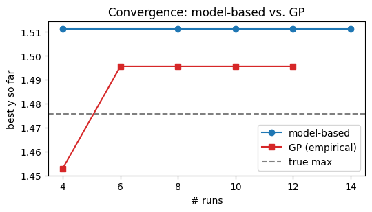
On this problem the model-based version typically reaches the
true maximum in 2-3 rounds, while the GP needs 5-10. The gap grows
with dimensionality and shrinks when the model form is wrong — if
you replace MichaelisMentenWithInhibition with the wrong functional
form, the model-based curve will plateau below the true maximum
while the GP eventually overtakes it.
7. Diagnostics worth checking#
Every round of model_based_optimize_round exposes:
result.parameters— the current MLE.result.parameter_se— standard errors from FIM⁻¹. A SE that’s large relative to the estimate is a warning sign that the data doesn’t constrain that parameter well; running an FIM-design round (optimal_experiment) on it would shrink it faster.result.fim_log_det— the D-optimality of the data set so far. Should grow monotonically; if it stalls, the new batch isn’t adding parameter information.result.incumbent_x/incumbent_y— best response so far.
8. Caveats#
Linearization of variance is exact only for models linear in parameters and asymptotically valid for nonlinear ones. For pathological posteriors (multimodal, heavy-tailed) you should upgrade to a Monte-Carlo propagation: sample \(\theta_s \sim \mathcal{N}(\hat\theta, \Sigma_\theta)\), evaluate \(f(d;\theta_s)\) for each, and use the empirical mean/std.
Initial guesses matter more than for GPs — a Gauss-Newton fit with a bad start can land in a flat local minimum. Either start from screening or from a coarse grid search.
Trust the model form, not the loop. If the residual ANOVA flags lack-of-fit (see
discopt.doe.anova_report), stop optimizing and go fix the model.