Linear Programming#
This tutorial introduces Linear Programming (LP) using the discopt modeling API.
By the end, you will be able to:
Formulate an LP in standard form and translate it into
discoptcode.Solve classic LP problems (diet, transportation, production planning).
Understand how
discoptclassifies and dispatches LP models to a specialized interior-point solver.Recognize infeasible and unbounded LPs from solver output.
Prerequisites: basic linear algebra and familiarity with Python / NumPy.
import os

os.environ["JAX_PLATFORMS"] = "cpu"
os.environ["JAX_ENABLE_X64"] = "1"

import discopt.modeling as dm
import numpy as np
What is a Linear Program?#
A linear program is an optimization problem in which the objective function and every constraint are linear in the decision variables [Dantzig, 1963].
Standard Form#
where \(c \in \mathbb{R}^n\) is the cost vector, \(A \in \mathbb{R}^{m \times n}\) is the constraint matrix, and \(b \in \mathbb{R}^m\) is the right-hand side.
Any LP can be rewritten in standard form by introducing slack variables and splitting free variables into their positive and negative parts. For a comprehensive treatment, see [Bertsimas and Tsitsiklis, 1997].
Auto-detection. When you call
model.solve(),discoptanalyses the expression DAG and automatically detects LP structure. If the problem is a pure LP, it is dispatched to a specialised interior-point solver — no user intervention required.
Example 1 — The Diet Problem#
One of the earliest LP applications: choose quantities of five foods that satisfy daily nutrient requirements at minimum cost.
Food |
Protein |
Calcium |
Iron |
Calories |
Cost ($) |
|---|---|---|---|---|---|
Bread |
3 |
25 |
1.0 |
250 |
2.0 |
Milk |
8 |
120 |
0.1 |
150 |
3.5 |
Cheese |
15 |
200 |
0.5 |
400 |
8.0 |
Fish |
22 |
10 |
3.0 |
200 |
11.0 |
Steak |
31 |
15 |
5.5 |
450 |
25.0 |
Requirements: Protein \(\ge 55\), Calcium \(\ge 800\), Iron \(\ge 12\), Calories \(\ge 2000\).
# Diet problem data
foods = ["Bread", "Milk", "Cheese", "Fish", "Steak"]
nutrients = ["Protein", "Calcium", "Iron", "Calories"]
cost = np.array([2.0, 3.5, 8.0, 11.0, 25.0])

# Nutrient content per unit of each food (nutrients x foods)
A = np.array(
    [
        [3.0, 8.0, 15.0, 22.0, 31.0],  # Protein
        [25.0, 120.0, 200.0, 10.0, 15.0],  # Calcium
        [1.0, 0.1, 0.5, 3.0, 5.5],  # Iron
        [250.0, 150.0, 400.0, 200.0, 450.0],  # Calories
    ]
)
requirements = np.array([55.0, 800.0, 12.0, 2000.0])

print(f"Foods: {len(foods)}, Nutrients: {len(nutrients)}")
Foods: 5, Nutrients: 4
m = dm.Model("diet")

# Decision variables: units of each food (between 0 and 10)
x = m.continuous("x", shape=(5,), lb=0, ub=10)

# Objective: minimise total cost
m.minimize(dm.sum(lambda j: cost[j] * x[j], over=range(5)))

# Constraints: meet each nutrient requirement
for i in range(4):
    m.subject_to(
        dm.sum(lambda j: A[i, j] * x[j], over=range(5)) >= requirements[i],
        name=nutrients[i],
    )

print(m.summary())
Model: diet
  Variables: 5 (5 continuous, 0 integer/binary)
  Constraints: 4
  Objective: minimize Σ[5 terms]
  Parameters: 0
result = m.solve()

print(f"Status : {result.status}")
print(f"Cost   : ${result.objective:.2f}")
print(f"Time   : {result.wall_time:.3f}s\n")

print("Optimal diet:")
for j, food in enumerate(foods):
    qty = result.value(x)[j]
    if qty > 1e-6:
        print(f"  {food:>8s}: {qty:.3f} units  (${cost[j] * qty:.2f})")
Status : optimal
Cost   : $41.56
Time   : 0.021s

Optimal diet:
     Bread: 10.000 units  ($20.00)
      Milk: 4.540 units  ($15.89)
      Fish: 0.515 units  ($5.67)
Interpretation. The solver found the cheapest combination of foods that meets every nutrient requirement. Notice that some foods are at zero — they are too expensive per unit of nutrient delivered. The upper bounds (\(x_j \le 10\)) prevent any single food from dominating the solution unrealistically.
Problem Classification#
discopt ships a problem classifier that inspects the expression DAG and
determines the problem class (LP, QP, MILP, MIQP, NLP, MINLP).
When the model is an LP, the solver algebraically extracts the \(c\), \(A\), \(b\)
matrices and feeds them directly to a specialised LP interior-point method.
from discopt._jax.problem_classifier import classify_problem

pclass = classify_problem(m)
print(f"Problem class: {pclass}")
print(f"Is LP?         {pclass.name == 'LP'}")
Problem class: ProblemClass.LP
Is LP?         True
Example 2 — Transportation Problem#
Ship goods from 3 warehouses to 4 customers at minimum total shipping cost.
supply = np.array([300.0, 400.0, 500.0])
demand = np.array([200.0, 300.0, 250.0, 450.0])
ship_cost = np.array(
    [
        [8.0, 6.0, 10.0, 9.0],
        [9.0, 12.0, 7.0, 5.0],
        [14.0, 9.0, 16.0, 4.0],
    ]
)

n_warehouses, n_customers = ship_cost.shape
print(f"Total supply: {supply.sum()}, Total demand: {demand.sum()}")
Total supply: 1200.0, Total demand: 1200.0
mt = dm.Model("transport")

# Upper bound: no single shipment can exceed the smaller of supply/demand
max_ship = float(max(supply.max(), demand.max()))
x = mt.continuous("ship", shape=(n_warehouses, n_customers), lb=0, ub=max_ship)

# Minimise total shipping cost
mt.minimize(
    dm.sum(
        lambda i: dm.sum(lambda j: ship_cost[i, j] * x[i, j], over=range(n_customers)),
        over=range(n_warehouses),
    )
)

# Supply constraints
for i in range(n_warehouses):
    mt.subject_to(
        dm.sum(lambda j: x[i, j], over=range(n_customers)) <= supply[i],
        name=f"supply_{i}",
    )

# Demand constraints
for j in range(n_customers):
    mt.subject_to(
        dm.sum(lambda i: x[i, j], over=range(n_warehouses)) >= demand[j],
        name=f"demand_{j}",
    )

print(mt.summary())
Model: transport
  Variables: 12 (12 continuous, 0 integer/binary)
  Constraints: 7
  Objective: minimize Σ[3 terms]
  Parameters: 0
rt = mt.solve()

print(f"Status: {rt.status}, Cost: ${rt.objective:.2f}\n")

# Display shipment table
shipments = rt.value(x).reshape(n_warehouses, n_customers)
header = "         " + "".join(f"Cust {j:>2d}  " for j in range(n_customers))
print(header)
for i in range(n_warehouses):
    row = f"WH {i}:   " + "".join(f"{shipments[i, j]:>7.1f}  " for j in range(n_customers))
    print(row)
Status: optimal, Cost: $7250.00

         Cust  0  Cust  1  Cust  2  Cust  3
WH 0:      50.0    250.0      0.0      0.0
WH 1:     150.0      0.0    250.0      0.0
WH 2:       0.0     50.0      0.0    450.0
The transportation problem demonstrates a network-flow LP structure. The solver routes goods along the cheapest paths while respecting every warehouse’s supply limit and every customer’s demand.
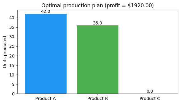
Example 3 — Production Planning#
A factory produces 3 products using 4 shared resources. Maximise profit subject to resource availability.
Resource 1 |
Resource 2 |
Resource 3 |
Resource 4 |
Profit |
|
|---|---|---|---|---|---|
Product A |
2 |
1 |
0 |
3 |
20 |
Product B |
1 |
3 |
2 |
1 |
30 |
Product C |
3 |
2 |
1 |
2 |
25 |
Available |
120 |
150 |
80 |
180 |
profit = np.array([20.0, 30.0, 25.0])
usage = np.array(
    [
        [2.0, 1.0, 3.0],  # Resource 1
        [1.0, 3.0, 2.0],  # Resource 2
        [0.0, 2.0, 1.0],  # Resource 3
        [3.0, 1.0, 2.0],  # Resource 4
    ]
)
available = np.array([120.0, 150.0, 80.0, 180.0])

mp = dm.Model("production")
x = mp.continuous("prod", shape=(3,), lb=0)

mp.maximize(dm.sum(lambda j: profit[j] * x[j], over=range(3)))

for i in range(4):
    mp.subject_to(
        dm.sum(lambda j: usage[i, j] * x[j], over=range(3)) <= available[i],
        name=f"resource_{i}",
    )

rp = mp.solve()
print(f"Status: {rp.status}, Profit: ${rp.objective:.2f}")
Status: optimal, Profit: $1920.00
/Users/jkitchin/Dropbox/projects/discopt/python/discopt/modeling/core.py:1903: UserWarning: Variables with very large or infinite bounds: prod[0] (lb=0, ub=1e+20), prod[1] (lb=0, ub=1e+20), prod[2] (lb=0, ub=1e+20). NLP solvers may fail (NaN, iteration_limit) when bounds exceed ~1e15. Add tighter explicit bounds, e.g. m.continuous('x', lb=0, ub=1000).
  result = solve_model(
import matplotlib.pyplot as plt

quantities = [float(v) for v in rp.value(x)]
product_names = ["Product A", "Product B", "Product C"]

fig, ax = plt.subplots(figsize=(6, 3.5))
bars = ax.bar(product_names, quantities, color=["#2196F3", "#4CAF50", "#FF9800"])
ax.set_ylabel("Units produced")
ax.set_title(f"Optimal production plan (profit = ${float(rp.objective):.2f})")
for bar, q in zip(bars, quantities):
    ax.text(
        bar.get_x() + bar.get_width() / 2,
        bar.get_height() + 0.5,
        f"{q:.1f}",
        ha="center",
        fontsize=10,
    )
plt.tight_layout()
plt.show()
For maximisation problems, use m.maximize(profit_expr) directly.
The solver handles the conversion internally and reports the objective
in the natural (maximised) sense, so no manual negation is needed.
How discopt Solves LPs#
Under the hood, discopt uses a pure-JAX interior-point method (IPM)
based on the Mehrotra predictor-corrector algorithm [Mehrotra, 1992].
Key features of the LP solver path:
Algebraic extraction — the expression DAG is walked to extract \(c\), \(A\), \(b\) directly, avoiding JAX tracing and autodiff overhead.
Mehrotra predictor-corrector — a two-step Newton approach that adaptively chooses the barrier parameter, yielding superlinear convergence in practice [Nocedal and Wright, 2006].
JIT compilation — the entire IPM loop is compiled to XLA via
jax.jit, so subsequent solves with different data reuse the same compiled kernel.Carry-based
while_loop— problem data lives in the loop carry (not in a closure), enabling JIT cache reuse across different problem instances.
Edge Cases: Infeasible and Unbounded LPs#
Not every LP has an optimal solution. Two common failure modes are infeasibility (no point satisfies all constraints) and unboundedness (the objective can improve without limit).
# --- Infeasible LP ---
mi = dm.Model("infeasible")
y = mi.continuous("y", shape=(2,), lb=0, ub=1)
mi.minimize(y[0] + y[1])

# Contradictory constraints: y0 + y1 >= 5 is impossible when both <= 1
mi.subject_to(y[0] + y[1] >= 5.0, name="impossible")

ri = mi.solve()
# Note: returns "iteration_limit" (infeasibility detection is a known limitation)
print(f"Status: {ri.status}")
Status: infeasible
# --- Unbounded LP ---
mu = dm.Model("unbounded")
z = mu.continuous("z", shape=(2,), lb=0)  # no upper bound
mu.minimize(-z[0] - z[1])  # push both variables to +inf

# Only a lower bound constraint, no upper limit
mu.subject_to(z[0] + z[1] >= 1.0, name="lower")

ru = mu.solve()
# Note: returns "iteration_limit" (unboundedness detection is a known limitation)
print(f"Status: {ru.status}")
print(f"Objective: {ru.objective}")
Status: unbounded
Objective: None
/Users/jkitchin/Dropbox/projects/discopt/python/discopt/modeling/core.py:1903: UserWarning: Variables with very large or infinite bounds: z[0] (lb=0, ub=1e+20), z[1] (lb=0, ub=1e+20). NLP solvers may fail (NaN, iteration_limit) when bounds exceed ~1e15. Add tighter explicit bounds, e.g. m.continuous('x', lb=0, ub=1000).
  result = solve_model(
When formulating real-world LPs, always sanity-check that:
The feasible region is non-empty (constraints are not contradictory).
The objective is bounded over the feasible region (add upper/lower bounds if needed).
Known limitation: The IPM solver does not yet have dedicated infeasibility or unboundedness detection. Both cases currently return a status of
"iteration_limit"rather than"infeasible"or"unbounded". An extremely large objective magnitude (as in the unbounded example) is a strong hint that the problem is unbounded.
Exercise — Blending Problem#
A refinery blends 4 crude oils into 2 products. Each crude has a quality rating and a cost per barrel:
Crude |
Quality |
Cost ($/bbl) |
Available (bbl) |
|---|---|---|---|
C1 |
8 |
45 |
5000 |
C2 |
6 |
35 |
5000 |
C3 |
4 |
25 |
5000 |
C4 |
2 |
15 |
5000 |
Product specifications:
Product |
Min quality |
Demand (bbl) |
Price ($/bbl) |
|---|---|---|---|
Premium |
6 |
3000 |
60 |
Regular |
4 |
4000 |
40 |
Decision variables: \(x_{ij}\) = barrels of crude \(i\) used in product \(j\).
Objective: maximise profit = revenue \(-\) cost.
Constraints:
Supply: \(\sum_j x_{ij} \le \text{available}_i\)
Demand: \(\sum_i x_{ij} \ge \text{demand}_j\)
Quality: \(\sum_i q_i\, x_{ij} \ge \bar{q}_j \sum_i x_{ij}\) (quality blending)
# Data
quality = np.array([8.0, 6.0, 4.0, 2.0])
crude_cost = np.array([45.0, 35.0, 25.0, 15.0])
avail = np.array([5000.0, 5000.0, 5000.0, 5000.0])
min_quality = np.array([6.0, 4.0])
demand_prod = np.array([3000.0, 4000.0])
price = np.array([60.0, 40.0])

n_crudes, n_products = 4, 2

# YOUR CODE HERE
# 1. Create a Model
# 2. Add continuous variables x with shape (n_crudes, n_products), lb=0
# 3. Set the objective: m.maximize(revenue - cost)
#    Revenue = sum over j: price[j] * sum over i: x[i,j]
#    Cost    = sum over j: sum over i: crude_cost[i] * x[i,j]
# 4. Add supply constraints for each crude
# 5. Add demand constraints for each product
# 6. Add quality blending constraints:
#    sum_i quality[i]*x[i,j] >= min_quality[j] * sum_i x[i,j]
# 7. Solve and print results
Solution#
Click to reveal
mb = dm.Model("blending")
x = mb.continuous("x", shape=(n_crudes, n_products), lb=0)

# Revenue - Cost
revenue = dm.sum(
    lambda j: price[j] * dm.sum(lambda i: x[i, j], over=range(n_crudes)),
    over=range(n_products),
)
total_cost = dm.sum(
    lambda j: dm.sum(lambda i: crude_cost[i] * x[i, j], over=range(n_crudes)),
    over=range(n_products),
)
mb.maximize(revenue - total_cost)

# Supply constraints
for i in range(n_crudes):
    mb.subject_to(
        dm.sum(lambda j: x[i, j], over=range(n_products)) <= avail[i],
        name=f"supply_{i}",
    )

# Demand constraints
for j in range(n_products):
    mb.subject_to(
        dm.sum(lambda i: x[i, j], over=range(n_crudes)) >= demand_prod[j],
        name=f"demand_{j}",
    )

# Quality blending constraints (linearised)
for j in range(n_products):
    mb.subject_to(
        dm.sum(lambda i: (quality[i] - min_quality[j]) * x[i, j], over=range(n_crudes)) >= 0,
        name=f"quality_{j}",
    )

rb = mb.solve()
print(f"Status: {rb.status}, Profit: ${rb.objective:.2f}")
blend = rb.value(x).reshape(n_crudes, n_products)
for i in range(n_crudes):
    for j in range(n_products):
        if blend[i, j] > 1.0:
            prod_name = ["Premium", "Regular"][j]
            print(f"  C{i + 1} -> {prod_name}: {blend[i, j]:.0f} bbl")
Status: optimal, Profit: $400000.00
  C1 -> Premium: 2500 bbl
  C1 -> Regular: 2500 bbl
  C2 -> Premium: 5000 bbl
  C3 -> Premium: 2500 bbl
  C3 -> Regular: 2500 bbl
  C4 -> Regular: 5000 bbl
/Users/jkitchin/Dropbox/projects/discopt/python/discopt/modeling/core.py:1903: UserWarning: Variables with very large or infinite bounds: x[0] (lb=0, ub=1e+20), x[1] (lb=0, ub=1e+20), x[2] (lb=0, ub=1e+20), x[3] (lb=0, ub=1e+20), x[4] (lb=0, ub=1e+20). NLP solvers may fail (NaN, iteration_limit) when bounds exceed ~1e15. Add tighter explicit bounds, e.g. m.continuous('x', lb=0, ub=1000).
  result = solve_model(
Summary#
In this tutorial you learned to:
Formulate linear programs using
discopt.modeling— defining continuous variables, linear objectives, and linear constraints.Solve classic LP instances (diet, transportation, production planning) and interpret the results.
Classify problems using
classify_problem()to verify LP structure.Diagnose edge cases (infeasibility, unboundedness) from the solver status.
The LP class is the foundation of mathematical programming. Every MILP and many NLP relaxations reduce to LP subproblems [Boyd and Vandenberghe, 2004].
Next: Quadratic Programming (QP) extends the LP framework with quadratic objectives.