Quadratic Programming#
This tutorial introduces Quadratic Programming (QP) – one of the most important problem classes in mathematical optimization. QPs appear throughout engineering, finance, statistics, and control theory.
By the end of this notebook you will be able to:
Define the standard form of a QP and explain why positive semi-definiteness of \(Q\) guarantees convexity.
Formulate three practical QPs in
discopt: portfolio optimization, ridge regression, and minimum-energy control.Understand how
discoptauto-detects QP structure and dispatches to a specialized interior-point solver.Trace out the efficient frontier of a Markowitz portfolio.
Prerequisites: basic linear algebra (matrix-vector products, eigenvalues) and familiarity with Python / NumPy. No prior optimization background is assumed.
References: [Boyd and Vandenberghe, 2004] is the standard graduate text on convex optimization, and Chapter 4 covers QPs in detail.
import os

os.environ["JAX_PLATFORMS"] = "cpu"
os.environ["JAX_ENABLE_X64"] = "1"

import discopt.modeling as dm
import numpy as np
1. What Is a Quadratic Program?#
A quadratic program (QP) is an optimization problem of the form
where
\(x \in \mathbb{R}^n\) is the vector of decision variables,
\(Q \in \mathbb{R}^{n \times n}\) is a symmetric matrix encoding the quadratic cost,
\(c \in \mathbb{R}^n\) is the linear cost vector,
\(A \in \mathbb{R}^{m \times n}\) and \(b \in \mathbb{R}^m\) define the inequality constraints.
Convexity and positive semi-definiteness#
The objective \(\tfrac{1}{2} x^\top Q\,x + c^\top x\) is convex if and only if \(Q\) is positive semi-definite (PSD), written \(Q \succeq 0\). Equivalently, all eigenvalues of \(Q\) are non-negative. When \(Q \succeq 0\), any local minimum is a global minimum, and efficient polynomial-time algorithms exist.
QP detection in discopt#
discopt automatically classifies your model by walking the expression DAG.
When it detects a quadratic objective with linear constraints and all
continuous variables, it dispatches to a specialized QP interior-point
method (IPM) [Mehrotra, 1992] that exploits the Schur complement
structure of the KKT system. This is dramatically faster than treating
the problem as a general NLP.
2. Example 1 – Markowitz Portfolio Optimization#
The mean-variance portfolio model [Markowitz, 1952] is perhaps the most famous QP. Given \(n\) assets with expected returns \(\mu \in \mathbb{R}^n\) and return covariance matrix \(\Sigma \in \mathbb{R}^{n \times n}\), we seek portfolio weights \(w \in \mathbb{R}^n\) that minimize risk (variance) for a target return:
This is a convex QP because \(\Sigma\) is positive semi-definite (it is a covariance matrix).
n_assets = 5
np.random.seed(42)

# Expected returns (annualized)
mu = np.array([0.12, 0.10, 0.07, 0.03, 0.15])

# Build a positive-definite covariance matrix via Cholesky factor
L = np.array(
    [
        [0.1, 0, 0, 0, 0],
        [0.02, 0.08, 0, 0, 0],
        [0.01, 0.01, 0.06, 0, 0],
        [0.005, 0.005, 0.005, 0.04, 0],
        [0.03, 0.02, 0.01, 0.005, 0.12],
    ]
)
Sigma = L @ L.T

print("Expected returns:", mu)
print("\nCovariance matrix:")
print(np.array2string(Sigma, precision=5))
print("\nEigenvalues of Sigma:", np.linalg.eigvalsh(Sigma))
print("All eigenvalues >= 0:", np.all(np.linalg.eigvalsh(Sigma) >= -1e-12))
Expected returns: [0.12 0.1  0.07 0.03 0.15]

Covariance matrix:
[[0.01    0.002   0.001   0.0005  0.003  ]
 [0.002   0.0068  0.001   0.0005  0.0022 ]
 [0.001   0.001   0.0038  0.0004  0.0011 ]
 [0.0005  0.0005  0.0004  0.00168 0.0005 ]
 [0.003   0.0022  0.0011  0.0005  0.01582]]

Eigenvalues of Sigma: [0.00157401 0.00348735 0.00587773 0.00911997 0.01804094]
All eigenvalues >= 0: True
target_return = 0.10

m = dm.Model("markowitz")
w = m.continuous("w", shape=(n_assets,), lb=0, ub=1)

# Objective: minimize portfolio variance  w' Sigma w
m.minimize(
    dm.sum(
        lambda i: dm.sum(
            lambda j: Sigma[i, j] * w[i] * w[j],
            over=range(n_assets),
        ),
        over=range(n_assets),
    )
)

# Constraints: weights sum to 1, minimum return
m.subject_to(dm.sum(w) == 1, name="budget")
m.subject_to(
    dm.sum(lambda i: mu[i] * w[i], over=range(n_assets)) >= target_return,
    name="min_return",
)

result = m.solve()
print(f"Status:    {result.status}")
print(f"Variance:  {result.objective:.6f}")
print(f"Weights:   {np.round(result.value(w), 4)}")
print(f"Return:    {np.dot(mu, result.value(w)):.4f}  (target: {target_return})")
Status:    optimal
Variance:  0.002809
Weights:   [0.2085 0.2431 0.305  0.0599 0.1835]
Return:    0.1000  (target: 0.1)
from discopt._jax.problem_classifier import classify_problem

# Verify that discopt detects this as a QP
problem_class = classify_problem(m)
print(f"Problem class: {problem_class}")
print("discopt routes this to the specialized QP-IPM solver.")
Problem class: ProblemClass.QP
discopt routes this to the specialized QP-IPM solver.
The efficient frontier#
By sweeping the target return \(r_{\min}\) from a low value to a high value and solving the QP at each point, we trace out the efficient frontier – the set of portfolios that achieve the lowest possible risk for each level of expected return. No rational investor would choose a portfolio below this curve, because a higher-return, same-risk alternative exists on it.
target_returns = np.linspace(0.04, 0.14, 10)
risks = []
achieved_returns = []

for r_target in target_returns:
    m = dm.Model("frontier")
    w = m.continuous("w", shape=(n_assets,), lb=0, ub=1)

    m.minimize(
        dm.sum(
            lambda i: dm.sum(
                lambda j: Sigma[i, j] * w[i] * w[j],
                over=range(n_assets),
            ),
            over=range(n_assets),
        )
    )
    m.subject_to(dm.sum(w) == 1, name="budget")
    m.subject_to(
        dm.sum(lambda i: mu[i] * w[i], over=range(n_assets)) >= r_target,
        name="min_return",
    )

    result = m.solve()
    if result.status in ("optimal", "feasible"):
        variance = result.objective
        risks.append(np.sqrt(max(variance, 0)))  # standard deviation
        achieved_returns.append(np.dot(mu, result.value(w)))
    else:
        print(f"  r_target={r_target:.2f}: {result.status}")

risks = np.array(risks)
achieved_returns = np.array(achieved_returns)
print(f"Computed {len(risks)} frontier points.")
Computed 10 frontier points.
import matplotlib.pyplot as plt

fig, ax = plt.subplots(figsize=(8, 5))
ax.plot(risks, achieved_returns, "o-", linewidth=2, markersize=6)
ax.set_xlabel("Risk (standard deviation)", fontsize=12)
ax.set_ylabel("Expected return", fontsize=12)
ax.set_title("Markowitz Efficient Frontier (5 assets)", fontsize=14)
ax.grid(True, alpha=0.3)
plt.tight_layout()
plt.show()
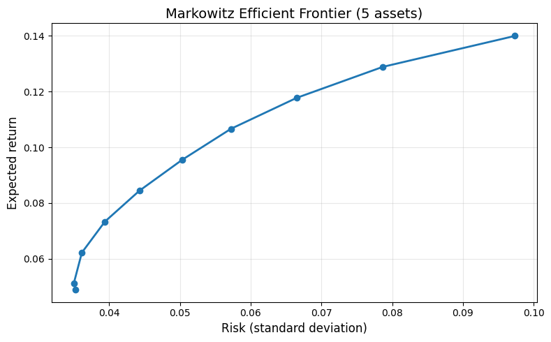
Interpretation. The curve bows to the left – as we demand higher returns, risk increases, but diversification keeps the curve concave. Points on the frontier dominate all portfolios to their right (same return, lower risk). This fundamental insight earned Harry Markowitz the Nobel Prize in Economics [Markowitz, 1952].
3. Example 2 – Ridge Regression as a QP#
Fitting a linear model \(\hat{y} = X\beta\) with \(L_2\) regularization (ridge regression) is secretly a QP [Boyd and Vandenberghe, 2004]:
Since \(X^\top X + \lambda I \succ 0\) for \(\lambda > 0\), this QP is strictly convex and has a unique solution. The closed-form solution is \(\beta^* = (X^\top X + \lambda I)^{-1} X^\top y\), which we will use to verify the optimizer’s answer.
np.random.seed(123)
n_samples, n_features = 50, 5

X = np.random.randn(n_samples, n_features)
true_beta = np.array([1.5, -2.0, 0.5, 0.0, 3.0])
y = X @ true_beta + 0.3 * np.random.randn(n_samples)

lam = 1.0  # regularization strength

print(f"Data: {n_samples} samples, {n_features} features")
print(f"True coefficients: {true_beta}")
print(f"Regularization lambda = {lam}")
Data: 50 samples, 5 features
True coefficients: [ 1.5 -2.   0.5  0.   3. ]
Regularization lambda = 1.0
m = dm.Model("ridge_regression")
beta = m.continuous("beta", shape=(n_features,), lb=-10, ub=10)

# Residual sum of squares: sum_i (y_i - sum_j X[i,j]*beta[j])^2
# + regularization: lambda * sum_j beta[j]^2
m.minimize(
    dm.sum(
        lambda i: (y[i] - dm.sum(lambda j: X[i, j] * beta[j], over=range(n_features))) ** 2,
        over=range(n_samples),
    )
    + lam * dm.sum(lambda j: beta[j] ** 2, over=range(n_features))
)

result = m.solve()
print(f"Status: {result.status}")
print(f"Objective (RSS + penalty): {result.objective:.4f}")
Status: optimal
Objective (RSS + penalty): 19.7872
# Closed-form ridge solution for verification
beta_cf = np.linalg.solve(X.T @ X + lam * np.eye(n_features), X.T @ y)
beta_opt = result.value(beta)

print(f"{'Coefficient':<14s} {'True':>8s} {'discopt':>10s} {'Closed-form':>12s}")
print("-" * 48)
for j in range(n_features):
    print(f"  beta[{j}]       {true_beta[j]:8.4f} {beta_opt[j]:10.4f} {beta_cf[j]:12.4f}")

max_error = np.max(np.abs(beta_opt - beta_cf))
print(f"\nMax |discopt - closed-form|: {max_error:.2e}")
Coefficient        True    discopt  Closed-form
------------------------------------------------
  beta[0]         1.5000     1.4290       1.4290
  beta[1]        -2.0000    -1.9478      -1.9478
  beta[2]         0.5000     0.4239       0.4239
  beta[3]         0.0000    -0.0034      -0.0034
  beta[4]         3.0000     2.9414       2.9414

Max |discopt - closed-form|: 5.10e-09
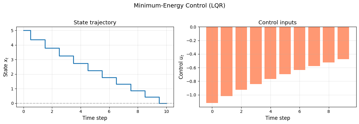
4. Example 3 – Minimum-Energy Control#
In discrete-time linear-quadratic regulator (LQR) problems we want to drive a system from an initial state \(x_0\) to the origin using minimum control energy. Consider the scalar system
with the objective
This is a QP in the controls \(u_t\) (and the auxiliary state variables \(x_t\)), with the dynamics as equality constraints [Boyd and Vandenberghe, 2004].
# System parameters
a, b = 1.1, 1.0  # slightly unstable open-loop system
T = 10  # horizon
x0 = 5.0  # initial state

m = dm.Model("lqr")
x = m.continuous("x", shape=(T + 1,), lb=-50, ub=50)  # states x[0]..x[T]
u = m.continuous("u", shape=(T,), lb=-10, ub=10)  # controls u[0]..u[T-1]

# Objective: minimize sum of squared controls
m.minimize(dm.sum(lambda t: u[t] ** 2, over=range(T)))

# Initial condition
m.subject_to(x[0] == x0, name="initial")

# Dynamics constraints: x[t+1] = a*x[t] + b*u[t]
for t in range(T):
    m.subject_to(x[t + 1] == a * x[t] + b * u[t], name=f"dynamics_{t}")

# Terminal constraint: drive state to zero
m.subject_to(x[T] == 0, name="terminal")

result = m.solve()
print(f"Status:    {result.status}")
print(f"Total energy (sum u^2): {result.objective:.4f}")
print(f"\nState trajectory:  {np.round(result.value(x), 3)}")
print(f"Control trajectory: {np.round(result.value(u), 3)}")
Status:    optimal
Total energy (sum u^2): 6.1666

State trajectory:  [5.    4.379 3.797 3.251 2.733 2.241 1.769 1.313 0.868 0.432 0.   ]
Control trajectory: [-1.121 -1.019 -0.927 -0.842 -0.766 -0.696 -0.633 -0.575 -0.523 -0.476]
fig, (ax1, ax2) = plt.subplots(1, 2, figsize=(12, 4))

times_x = np.arange(T + 1)
times_u = np.arange(T)

ax1.step(times_x, result.value(x), where="mid", linewidth=2)
ax1.axhline(0, color="gray", linestyle="--", alpha=0.5)
ax1.set_xlabel("Time step", fontsize=12)
ax1.set_ylabel("State $x_t$", fontsize=12)
ax1.set_title("State trajectory", fontsize=13)
ax1.grid(True, alpha=0.3)

ax2.bar(times_u, result.value(u), color="coral", alpha=0.8)
ax2.axhline(0, color="gray", linestyle="--", alpha=0.5)
ax2.set_xlabel("Time step", fontsize=12)
ax2.set_ylabel("Control $u_t$", fontsize=12)
ax2.set_title("Control inputs", fontsize=13)
ax2.grid(True, alpha=0.3)

plt.suptitle("Minimum-Energy Control (LQR)", fontsize=14, y=1.02)
plt.tight_layout()
plt.show()
5. How discopt Solves QPs#
When discopt detects a QP, it follows a specialized path:
Algebraic coefficient extraction. Instead of using automatic differentiation (which would require \(O(n^2)\) Hessian evaluations),
discoptwalks the expression DAG to directly extract the \(Q\) matrix, linear cost vector \(c\), and constraint matrix \(A\). This is 100–200x faster than the autodiff path.Carry-based IPM. The extracted data is fed into a Mehrotra predictor-corrector interior-point method [Mehrotra, 1992] that stores all problem data in the
while_loopcarry state (rather than in closures), enabling JIT cache reuse across different problem instances of the same size.Schur complement. The KKT system \(\begin{bmatrix} Q + \delta_p I & A^\top \\ A & -\delta_d I \end{bmatrix}\) is reduced via the Schur complement and solved with a Cholesky factorization, exploiting the block structure for efficiency.
Bulk API. For large-scale QPs where building the objective
expression-by-expression would be slow, discopt provides
add_quadratic_objective(Q, c, x) which accepts the \(Q\) matrix and
\(c\) vector directly, bypassing DAG construction entirely.
For active-set methods as an alternative to IPM, see [Goldfarb and Idnani, 1983]. For a comprehensive treatment of numerical optimization algorithms, see [Nocedal and Wright, 2006].
from discopt._jax.problem_classifier import classify_problem, extract_qp_data_algebraic

# Rebuild a small portfolio QP to inspect extracted data
m = dm.Model("qp_inspect")
w = m.continuous("w", shape=(3,), lb=0, ub=1)
Sigma3 = Sigma[:3, :3]

m.minimize(
    dm.sum(
        lambda i: dm.sum(
            lambda j: Sigma3[i, j] * w[i] * w[j],
            over=range(3),
        ),
        over=range(3),
    )
)
m.subject_to(dm.sum(w) == 1, name="budget")

pc = classify_problem(m)
print(f"Detected class: {pc}")

qp_data = extract_qp_data_algebraic(m)
print("\nQ matrix (Hessian of objective):")
print(np.array2string(np.array(qp_data.Q), precision=5))
print(f"\nc vector (linear cost): {np.array(qp_data.c)}")
Detected class: ProblemClass.QP

Q matrix (Hessian of objective):
[[0.02   0.004  0.002 ]
 [0.004  0.0136 0.002 ]
 [0.002  0.002  0.0076]]

c vector (linear cost): [0. 0. 0.]
6. Non-convex QPs: A Warning#
When \(Q\) has negative eigenvalues (i.e., \(Q\) is not PSD), the QP is non-convex. The objective has saddle points and potentially multiple local minima. A local solver may return a local (not global) optimum.
Below we maximize a quadratic using m.maximize(), which internally
corresponds to a negative-definite \(Q\).
m = dm.Model("non_convex_qp")
x = m.continuous("x", lb=-5, ub=5)
y = m.continuous("y", lb=-5, ub=5)

# Maximizing x^2 + y^2: non-convex!
m.maximize(x**2 + y**2)
m.subject_to(x + y <= 6)

result = m.solve()
print(f"Status:    {result.status}")
print(f"Objective: {result.objective:.4f}")
print(f"x = {result.value(x):.4f}")
print(f"y = {result.value(y):.4f}")
print()
print("Note: The global maximum of x^2 + y^2 on [-5,5]^2 is 50")
print("at a corner (5, -5) or (-5, 5), etc.")
print("A local solver may find a different local optimum.")
Status:    optimal
Objective: 18.0000
x = 3.0000
y = 3.0000

Note: The global maximum of x^2 + y^2 on [-5,5]^2 is 50
at a corner (5, -5) or (-5, 5), etc.
A local solver may find a different local optimum.
7. Exercise: SVM Dual as a QP#
The dual of a support vector machine (SVM) for binary classification is a classic QP. Given \(m\) training points \((x_i, y_i)\) with \(y_i \in \{-1, +1\}\), the dual SVM is:
This is a concave maximization (equivalently, convex minimization by negation) because the kernel matrix \(K_{ij} = y_i y_j x_i^\top x_j\) is positive semi-definite.
Task: Complete the code below to solve the dual SVM on a toy 2D dataset.
# Generate a simple linearly separable 2D dataset
np.random.seed(7)
n_pos = 15
n_neg = 15
n_total = n_pos + n_neg

X_pos = np.random.randn(n_pos, 2) + np.array([2.0, 2.0])
X_neg = np.random.randn(n_neg, 2) + np.array([-2.0, -2.0])
X_data = np.vstack([X_pos, X_neg])
y_labels = np.concatenate([np.ones(n_pos), -np.ones(n_neg)])

C = 10.0  # regularization parameter

# Kernel matrix
K = np.zeros((n_total, n_total))
for i in range(n_total):
    for j in range(n_total):
        K[i, j] = y_labels[i] * y_labels[j] * np.dot(X_data[i], X_data[j])

# --- YOUR CODE HERE ---
# 1. Create a Model
# 2. Add alpha variables with lb=0, ub=C
# 3. Maximize: sum(alpha) - 0.5 * sum_ij alpha_i * alpha_j * K[i,j]
#    (Hint: use m.maximize(...))
# 4. Add constraint: sum_i alpha_i * y_labels[i] == 0
# 5. Solve and print results
# --- END YOUR CODE ---
# --- SOLUTION ---
m = dm.Model("svm_dual")
alpha = m.continuous("alpha", shape=(n_total,), lb=0, ub=C)

# Maximize the dual SVM objective
m.maximize(
    dm.sum(alpha)
    - 0.5
    * dm.sum(
        lambda i: dm.sum(
            lambda j: K[i, j] * alpha[i] * alpha[j],
            over=range(n_total),
        ),
        over=range(n_total),
    )
)

# Equality constraint: sum of alpha_i * y_i = 0
m.subject_to(dm.sum(lambda i: y_labels[i] * alpha[i], over=range(n_total)) == 0, name="balance")

result = m.solve()
print(f"Status: {result.status}")
print(f"Objective: {result.objective:.4f}")

alpha_vals = result.value(alpha)
# Support vectors have alpha > small threshold
sv_mask = alpha_vals > 1e-4
print(f"Number of support vectors: {np.sum(sv_mask)} / {n_total}")
print(f"Support vector indices: {np.where(sv_mask)[0]}")
Status: optimal
Objective: 0.4015
Number of support vectors: 3 / 30
Support vector indices: [13 23 25]
8. Summary#
In this tutorial we covered:
Topic |
Key takeaway |
|---|---|
QP standard form |
\(\min \tfrac{1}{2} x^\top Q x + c^\top x\) s.t. \(Ax \le b\) |
Convexity |
\(Q \succeq 0\) (PSD) guarantees a unique global minimum |
Portfolio optimization |
Markowitz mean-variance is a QP; efficient frontier from parametric solves [Markowitz, 1952] |
Ridge regression |
\(L_2\)-regularized least squares is a QP with \(Q = X^\top X + \lambda I\) |
Minimum-energy control |
LQR with linear dynamics yields a QP in controls |
Algebraic extraction |
|
Non-convex QPs |
Indefinite \(Q\) leads to non-convex problems; local solvers may miss the global optimum |
Next steps#
Mixed-integer QP (MIQP): Add binary variables to the portfolio model (e.g., cardinality constraints) – see
tutorial_miqp.Mixed-integer LP (MILP): When the objective is linear – see
tutorial_milp.Nonlinear programming (NLP): For general smooth objectives – see
tutorial_minlp.