Dynamic Optimization with DAE Collocation

Many engineering problems involve dynamics — systems that evolve over time according to differential equations. Examples include:

• Optimal control: find inputs that drive a system to a desired state with minimum cost

• Parameter estimation: fit kinetic parameters to experimental time-series data

• Experiment design: choose operating conditions to maximize information content

• PDE-constrained optimization: optimize systems governed by partial differential equations

The discopt.dae module transcribes ODE/DAE systems into algebraic constraints using orthogonal collocation on finite elements [Biegler, 2010] or finite differences, enabling these problems to be solved as standard NLPs within discopt’s existing solver infrastructure.

This tutorial covers:

1. Orthogonal collocation background

2. First-order ODEs (exponential decay, chemical kinetics)

3. Parameter estimation from experimental data

4. Optimal control with piecewise-constant controls

5. Second-order ODEs (harmonic oscillator)

6. Index-1 DAEs (algebraic constraints)

7. Method of lines for 1D PDEs

8. Finite-difference discretization

%matplotlib inline

import os

os.environ["JAX_PLATFORMS"] = "cpu"
os.environ["JAX_ENABLE_X64"] = "1"

import matplotlib.pyplot as plt
import numpy as np
from discopt import Model
from discopt.dae import (
    ContinuousSet,
    DAEBuilder,
    FDBuilder,
    align_time_grid,
    collocation_matrix,
    legendre_roots,
    radau_roots,
)

print("All imports successful")

All imports successful

1. Orthogonal Collocation Background

Orthogonal collocation on finite elements [Biegler, 2010] is the workhorse method for transcribing ODE/DAE systems into algebraic constraints suitable for NLP solvers. The idea is to divide the time horizon \([t_0, t_f]\) into \(N_{fe}\) finite elements, and within each element approximate the state trajectory as a polynomial that passes through selected collocation points.

Collocation schemes

Two families of collocation points are commonly used:

• Radau IIA: Points are the roots of a shifted Radau polynomial on \([0, 1]\). The last point is always \(\tau = 1\) (the element boundary), which provides automatic \(C^0\) continuity between elements. This is the default in discopt.

• Gauss–Legendre: Points are the roots of a Legendre polynomial mapped to \((0, 1)\). Neither endpoint is included, giving higher-order accuracy but requiring explicit continuity constraints.

Differentiation matrix

Given the full node set \([0, \tau_1, \ldots, \tau_{n_{cp}}]\) (element start plus collocation points), the differentiation matrix \(A \in \mathbb{R}^{n_{cp} \times (n_{cp}+1)}\) maps function values at all nodes to derivative values at the collocation points:

\[A_{jk} = L_k'(\tau_j)\]

where \(L_k\) is the \(k\)-th Lagrange basis polynomial through the full node set. The collocation equation for state \(x\) in element \(i\) at collocation point \(j\) is:

\[\sum_{k=0}^{n_{cp}} A_{jk} \, x_{i,k} = h_i \, f(t_{i,j}, x_{i,j})\]

where \(h_i\) is the element width and \(f\) is the ODE right-hand side [Cuthrell and Biegler, 1987].

Let’s inspect the collocation points and differentiation matrices.

# Radau IIA roots for different numbers of collocation points
for ncp in range(1, 6):
    roots = radau_roots(ncp)
    print(f"Radau ncp={ncp}: {np.array2string(roots, precision=6)}")

print()

# Gauss-Legendre roots
for ncp in range(1, 5):
    roots = legendre_roots(ncp)
    print(f"Legendre ncp={ncp}: {np.array2string(roots, precision=6)}")

print()

# Differentiation matrix for Radau with 3 collocation points
A, w = collocation_matrix(3, "radau")
print("Differentiation matrix A (Radau, ncp=3):")
print(np.array2string(A, precision=4, suppress_small=True))
print(f"\nContinuity weights w: {np.array2string(w, precision=4)}")
print(f"A shape: {A.shape}  (ncp x (ncp+1))")

Radau ncp=1: [1.]
Radau ncp=2: [0.333333 1.      ]
Radau ncp=3: [0.155051 0.644949 1.      ]
Radau ncp=4: [0.088588 0.409467 0.787659 1.      ]
Radau ncp=5: [0.057104 0.276843 0.58359  0.86024  1.      ]

Legendre ncp=1: [0.5]
Legendre ncp=2: [0.211325 0.788675]
Legendre ncp=3: [0.112702 0.5      0.887298]
Legendre ncp=4: [0.069432 0.330009 0.669991 0.930568]

Differentiation matrix A (Radau, ncp=3):
[[-4.1394  3.2247  1.1678 -0.2532]
 [ 1.7394 -3.5678  0.7753  1.0532]
 [-3.      5.532  -7.532   5.    ]]

Continuity weights w: [-0.  0. -0.  1.]
A shape: (3, 4)  (ncp x (ncp+1))

2. First-Order ODEs: Exponential Decay

We start with the simplest possible ODE — exponential decay:

\[\frac{dx}{dt} = -x, \quad x(0) = 1\]

The exact solution is \(x(t) = e^{-t}\). We’ll solve this as a feasibility problem (no objective) and compare the collocation solution with the analytical result.

The workflow with DAEBuilder is:

1. Create a Model and a ContinuousSet (time domain + discretization parameters)

2. Create a DAEBuilder and declare states with add_state()

3. Define the ODE right-hand side with set_ode()

4. Call discretize() to generate all variables and constraints

5. Solve and extract the solution

# Model setup
m = Model("exp_decay")
cs = ContinuousSet("t", bounds=(0, 5), nfe=10, ncp=3, scheme="radau")
dae = DAEBuilder(m, cs)

# Declare state with initial condition
dae.add_state("x", initial=1.0, bounds=(0, 2))

# ODE: dx/dt = -x
dae.set_ode(lambda t, states, alg, ctrl: {"x": -states["x"]})

# Discretize and solve (minimize 0 = feasibility problem)
dae.discretize()
m.minimize(0)
result = m.solve()

print(f"Status: {result.status}")

# Extract and plot
t_num, x_num = dae.extract_solution(result, "x")
t_exact = np.linspace(0, 5, 200)
x_exact = np.exp(-t_exact)

fig, (ax1, ax2) = plt.subplots(1, 2, figsize=(10, 4))

ax1.plot(t_exact, x_exact, "k-", label="Exact: $e^{-t}$", linewidth=2)
ax1.plot(t_num, x_num, "ro", markersize=5, label=f"Collocation ({cs.nfe} elements, {cs.ncp} cp)")
ax1.set_xlabel("t")
ax1.set_ylabel("x(t)")
ax1.set_title("Exponential Decay")
ax1.legend()

# Error plot
x_exact_at_nodes = np.exp(-t_num)
error = np.abs(x_num - x_exact_at_nodes)
ax2.semilogy(t_num, error, "bo-", markersize=4)
ax2.set_xlabel("t")
ax2.set_ylabel("Absolute error")
ax2.set_title("Collocation Error")
ax2.grid(True, alpha=0.3)

plt.tight_layout()
plt.show()

max_err = np.max(error)
print(f"Max absolute error: {max_err:.2e}")

******************************************************************************
This program contains Ipopt, a library for large-scale nonlinear optimization.
 Ipopt is released as open source code under the Eclipse Public License (EPL).
         For more information visit https://github.com/coin-or/Ipopt
******************************************************************************

Status: optimal

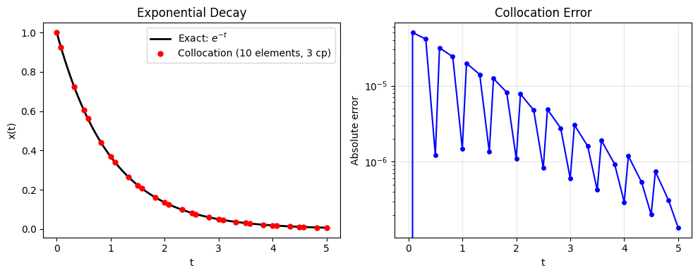
Max absolute error: 5.00e-05

3. Two-Species Chemical Kinetics

Consider a series reaction \(A \xrightarrow{k_1} B \xrightarrow{k_2} C\) governed by:

\[\frac{dA}{dt} = -k_1 A, \qquad \frac{dB}{dt} = k_1 A - k_2 B\]

with initial conditions \(A(0) = 1\), \(B(0) = 0\) and rate constants \(k_1 = 2\), \(k_2 = 1\).

The analytical solution is:

\[A(t) = e^{-k_1 t}, \qquad B(t) = \frac{k_1}{k_2 - k_1}\left(e^{-k_1 t} - e^{-k_2 t}\right)\]

This example demonstrates multiple coupled states in the set_ode() callback.

k1, k2 = 2.0, 1.0

m = Model("kinetics")
cs = ContinuousSet("t", bounds=(0, 5), nfe=15, ncp=3)
dae = DAEBuilder(m, cs)

dae.add_state("A", initial=1.0, bounds=(0, 2))
dae.add_state("B", initial=0.0, bounds=(0, 2))


def kinetics_rhs(t, states, alg, ctrl):
    A = states["A"]
    B = states["B"]
    return {
        "A": -k1 * A,
        "B": k1 * A - k2 * B,
    }


dae.set_ode(kinetics_rhs)
dae.discretize()
m.minimize(0)
result = m.solve()

print(f"Status: {result.status}")

t_A, A_num = dae.extract_solution(result, "A")
t_B, B_num = dae.extract_solution(result, "B")

# Analytical solutions
t_exact = np.linspace(0, 5, 200)
A_exact = np.exp(-k1 * t_exact)
B_exact = k1 / (k2 - k1) * (np.exp(-k1 * t_exact) - np.exp(-k2 * t_exact))

plt.figure(figsize=(8, 5))
plt.plot(t_exact, A_exact, "b-", linewidth=2, label="A (exact)")
plt.plot(t_exact, B_exact, "r-", linewidth=2, label="B (exact)")
plt.plot(t_A, A_num, "bs", markersize=5, label="A (collocation)")
plt.plot(t_B, B_num, "ro", markersize=5, label="B (collocation)")
plt.xlabel("t")
plt.ylabel("Concentration")
plt.title("Series Reaction $A \\to B \\to C$")
plt.legend()
plt.grid(True, alpha=0.3)
plt.show()

# Check errors
A_exact_nodes = np.exp(-k1 * t_A)
B_exact_nodes = k1 / (k2 - k1) * (np.exp(-k1 * t_B) - np.exp(-k2 * t_B))
print(f"Max error A: {np.max(np.abs(A_num - A_exact_nodes)):.2e}")
print(f"Max error B: {np.max(np.abs(B_num - B_exact_nodes)):.2e}")

Status: optimal

Max error A: 1.41e-04
Max error B: 2.60e-04

4. Parameter Estimation

A common application of dynamic optimization is parameter estimation: given noisy experimental data, find the model parameters that best fit the observations.

We’ll estimate the decay rate \(k\) from noisy measurements of exponential decay \(dx/dt = -kx\), \(x(0) = 1\). The true value is \(k = 0.5\).

The optimization problem is:

\[\min_{k, x(\cdot)} \sum_{i} \left(x(t_i) - \hat{x}_i\right)^2 \quad \text{s.t.} \quad \frac{dx}{dt} = -kx, \; x(0) = 1\]

where \(\hat{x}_i\) are the noisy measurements at times \(t_i\).

Two convenience utilities simplify this workflow:

• align_time_grid() adjusts element boundaries so measurement times coincide with element boundaries (where collocation nodes exist).

• DAEBuilder.least_squares() builds the sum-of-squared-residuals objective by mapping each measurement to the nearest collocation node.

# Generate synthetic noisy data
k_true = 0.5
np.random.seed(42)
t_data = np.array([0.5, 1.0, 1.5, 2.0, 3.0, 4.0, 5.0])
x_data = np.exp(-k_true * t_data) + 0.02 * np.random.randn(len(t_data))

# Align the time grid so element boundaries include measurement times
eb = align_time_grid(t_span=(0, 5), nfe=20, measurement_times=t_data)
print(f"Aligned grid: {len(eb) - 1} elements")

# Build the estimation problem
m = Model("param_estimation")
cs = ContinuousSet("t", bounds=(0, 5), nfe=len(eb) - 1, ncp=3, element_boundaries=eb)
dae = DAEBuilder(m, cs)

dae.add_state("x", initial=1.0, bounds=(0, 2))

# k is a free parameter to estimate
k = m.continuous("k", lb=0.01, ub=5.0)

# ODE: dx/dt = -k*x (k is a model variable, not a Python constant)
dae.set_ode(lambda t, states, alg, ctrl: {"x": -k * states["x"]})
dae.discretize()

# Build least-squares objective using the convenience method
m.minimize(dae.least_squares("x", t_data, x_data))

result = m.solve()

k_est = result.value(k)
print(f"Status: {result.status}")
print(f"Estimated k: {k_est:.4f}  (true: {k_true})")
print(f"Relative error: {abs(k_est - k_true) / k_true * 100:.2f}%")

# Plot fit vs data
t_sol, x_sol = dae.extract_solution(result, "x")
t_fine = np.linspace(0, 5, 200)

plt.figure(figsize=(8, 5))
plt.plot(t_fine, np.exp(-k_true * t_fine), "k--", linewidth=1.5, label=f"True ($k={k_true}$)")
plt.plot(t_sol, x_sol, "b-", linewidth=2, label=f"Estimated ($k={k_est:.3f}$)")
plt.plot(t_data, x_data, "ro", markersize=8, label="Noisy data")
plt.xlabel("t")
plt.ylabel("x(t)")
plt.title("Parameter Estimation: Exponential Decay")
plt.legend()
plt.grid(True, alpha=0.3)
plt.show()

Aligned grid: 20 elements

Status: optimal
Estimated k: 0.4836  (true: 0.5)
Relative error: 3.27%

5. Optimal Control

In optimal control, we seek an input (control) trajectory \(u(t)\) that drives a dynamic system to achieve some objective. Consider the linear system:

\[\frac{dx}{dt} = -x + u, \quad x(0) = 1\]

with the objective of minimizing integrated control effort plus a terminal penalty:

\[\min \int_0^5 u^2 \, dt + 10 \cdot x(5)^2\]

The control \(u\) is piecewise constant over each finite element, declared via add_control(). The integral is computed using the collocation quadrature weights via dae.integral() [Betts, 2010].

m = Model("optimal_control")
cs = ContinuousSet("t", bounds=(0, 5), nfe=20, ncp=3)
dae = DAEBuilder(m, cs)

dae.add_state("x", initial=1.0, bounds=(-5, 5))
dae.add_control("u", bounds=(-2, 2))

# ODE: dx/dt = -x + u
dae.set_ode(lambda t, states, alg, ctrl: {"x": -states["x"] + ctrl["u"]})
dae.discretize()

# Objective: integral of u^2 + terminal penalty on x(tf)
integral_cost = dae.integral(lambda t, s, a, c: c["u"] ** 2)

x_var = dae.get_state("x")
terminal_penalty = 10.0 * x_var[-1, -1] ** 2

m.minimize(integral_cost + terminal_penalty)

result = m.solve()
print(f"Status: {result.status}")
print(f"Objective: {result.objective:.4f}")

# Extract solution
t_x, x_sol = dae.extract_solution(result, "x")
u_var = dae.get_state("u")
u_sol = result.value(u_var)

# Control is piecewise constant: one value per element
t0, tf = cs.bounds
h = (tf - t0) / cs.nfe
t_u_edges = np.array([t0 + i * h for i in range(cs.nfe + 1)])

fig, (ax1, ax2) = plt.subplots(2, 1, figsize=(8, 6), sharex=True)

ax1.plot(t_x, x_sol, "b-o", markersize=3, linewidth=1.5, label="x(t)")
ax1.axhline(y=0, color="gray", linestyle="--", alpha=0.5)
ax1.set_ylabel("State x(t)")
ax1.set_title("Optimal Control: $dx/dt = -x + u$")
ax1.legend()
ax1.grid(True, alpha=0.3)

# Plot piecewise constant control as step function
for i in range(cs.nfe):
    ax2.plot([t_u_edges[i], t_u_edges[i + 1]], [u_sol[i], u_sol[i]], "r-", linewidth=2)
    if i < cs.nfe - 1:
        ax2.plot(
            [t_u_edges[i + 1], t_u_edges[i + 1]], [u_sol[i], u_sol[i + 1]], "r:", linewidth=0.5
        )

ax2.set_xlabel("t")
ax2.set_ylabel("Control u(t)")
ax2.legend(["u(t)"])
ax2.grid(True, alpha=0.3)

plt.tight_layout()
plt.show()

print(f"Terminal state x(5) = {x_sol[-1]:.6f}")
print(f"Terminal penalty: {10 * x_sol[-1] ** 2:.6f}")

Status: optimal
Objective: 0.0001

Terminal state x(5) = 0.001128
Terminal penalty: 0.000013

6. Second-Order ODEs: Harmonic Oscillator

Many physical systems are naturally described by second-order ODEs. The harmonic oscillator is:

\[\frac{d^2 x}{dt^2} = -x, \quad x(0) = 1, \; \dot{x}(0) = 0\]

with exact solution \(x(t) = \cos(t)\).

The add_second_order_state() method automatically introduces a velocity variable and the coupling \(dx/dt = v\). The user only needs to supply the acceleration via set_second_order_ode().

m = Model("harmonic_oscillator")
cs = ContinuousSet("t", bounds=(0, 4 * np.pi), nfe=40, ncp=3)
dae = DAEBuilder(m, cs)

# Second-order state: position x, automatically creates velocity dx_dt
dae.add_second_order_state(
    "x",
    initial=1.0,  # x(0) = 1
    initial_velocity=0.0,  # dx/dt(0) = 0
    bounds=(-2, 2),
    velocity_bounds=(-2, 2),
)

# Acceleration: d^2x/dt^2 = -x
dae.set_second_order_ode(lambda t, pos, vel, alg, ctrl: {"x": -pos["x"]})

dae.discretize()
m.minimize(0)
result = m.solve()

print(f"Status: {result.status}")

# Extract position and velocity
t_x, x_sol = dae.extract_solution(result, "x")
t_v, v_sol = dae.extract_solution(result, "dx_dt")

t_exact = np.linspace(0, 4 * np.pi, 500)

fig, (ax1, ax2) = plt.subplots(2, 1, figsize=(10, 6), sharex=True)

ax1.plot(t_exact, np.cos(t_exact), "k-", linewidth=2, label="Exact: $\\cos(t)$")
ax1.plot(t_x, x_sol, "ro", markersize=3, label="Collocation")
ax1.set_ylabel("Position x(t)")
ax1.set_title("Harmonic Oscillator: $d^2x/dt^2 = -x$")
ax1.legend()
ax1.grid(True, alpha=0.3)

ax2.plot(t_exact, -np.sin(t_exact), "k-", linewidth=2, label="Exact: $-\\sin(t)$")
ax2.plot(t_v, v_sol, "bo", markersize=3, label="Collocation")
ax2.set_xlabel("t")
ax2.set_ylabel("Velocity $dx/dt$")
ax2.legend()
ax2.grid(True, alpha=0.3)

plt.tight_layout()
plt.show()

x_exact_nodes = np.cos(t_x)
print(f"Max position error: {np.max(np.abs(x_sol - x_exact_nodes)):.2e}")

Status: optimal

Max position error: 1.32e-05

7. Index-1 DAE

A differential-algebraic equation (DAE) couples differential states \(x\) with algebraic variables \(z\) that satisfy algebraic (non-differential) constraints. An index-1 DAE has the form:

\[\frac{dx}{dt} = f(x, z), \qquad 0 = g(x, z)\]

where the Jacobian \(\partial g / \partial z\) is nonsingular.

Consider the system:

\[\frac{dx}{dt} = -x + z, \qquad 0 = x^2 - z\]

The algebraic constraint forces \(z = x^2\) at all times, so the ODE reduces to \(dx/dt = -x + x^2\), which is a Bernoulli equation with known solution.

With DAEBuilder, algebraic variables are declared via add_algebraic() and the algebraic equations via set_algebraic(). Algebraic variables exist only at collocation points (not at element boundaries) [Biegler, 2010].

m = Model("index1_dae")
cs = ContinuousSet("t", bounds=(0, 3), nfe=20, ncp=3)
dae = DAEBuilder(m, cs)

dae.add_state("x", initial=0.5, bounds=(0, 2))
dae.add_algebraic("z", bounds=(0, 4))

# ODE: dx/dt = -x + z
dae.set_ode(lambda t, s, a, c: {"x": -s["x"] + a["z"]})

# Algebraic: 0 = x^2 - z
dae.set_algebraic(lambda t, s, a, c: {"z": s["x"] ** 2 - a["z"]})

dae.discretize()
m.minimize(0)
result = m.solve()

print(f"Status: {result.status}")

t_x, x_sol = dae.extract_solution(result, "x")

# Exact solution: dx/dt = -x + x^2 is a Bernoulli equation.
# With substitution y = 1/x: dy/dt = 1 - y, y(0) = 1/x(0) = 2
# y(t) = 1 + (y0 - 1)*exp(-t) = 1 + exp(-t)
# x(t) = 1 / (1 + exp(-t))
x0 = 0.5
y0 = 1.0 / x0
t_fine = np.linspace(0, 3, 200)
y_exact = 1.0 + (y0 - 1.0) * np.exp(-t_fine)
x_exact = 1.0 / y_exact
z_exact = x_exact**2

fig, (ax1, ax2) = plt.subplots(1, 2, figsize=(10, 4))

ax1.plot(t_fine, x_exact, "k-", linewidth=2, label="Exact x(t)")
ax1.plot(t_x, x_sol, "ro", markersize=4, label="Collocation x(t)")
ax1.plot(t_fine, z_exact, "b--", linewidth=2, label="Exact z(t) = x(t)$^2$")
ax1.set_xlabel("t")
ax1.set_ylabel("Value")
ax1.set_title("Index-1 DAE: $dx/dt = -x + z$, $0 = x^2 - z$")
ax1.legend()
ax1.grid(True, alpha=0.3)

# Verify algebraic constraint holds
y_exact_nodes = 1.0 + (y0 - 1.0) * np.exp(-t_x)
x_exact_nodes = 1.0 / y_exact_nodes
error = np.abs(x_sol - x_exact_nodes)

ax2.semilogy(t_x, error, "bo-", markersize=3)
ax2.set_xlabel("t")
ax2.set_ylabel("Absolute error")
ax2.set_title("DAE Solution Error")
ax2.grid(True, alpha=0.3)

plt.tight_layout()
plt.show()

print(f"Max error in x: {np.max(error):.2e}")

Status: optimal

Max error in x: 9.05e-01

8. Method of Lines: 1D Heat Equation

The method of lines (MOL) converts a PDE into a system of ODEs by discretizing the spatial domain and leaving the time domain continuous. For the 1D heat equation:

\[\frac{\partial T}{\partial t} = \alpha \frac{\partial^2 T}{\partial x^2}, \quad T(0,t) = 0, \; T(1,t) = 0, \; T(x,0) = \sin(\pi x)\]

we discretize the spatial domain \([0, 1]\) into \(N\) interior points using central differences for \(\partial^2 T / \partial x^2\), yielding an ODE system:

\[\frac{dT_i}{dt} = \alpha \frac{T_{i-1} - 2T_i + T_{i+1}}{\Delta x^2}\]

with \(T_0 = T_{N+1} = 0\) (boundary conditions).

The n_components parameter in add_state() lets us represent the spatial grid as a vector-valued state.

alpha = 0.1  # thermal diffusivity
N = 10  # interior spatial points
dx = 1.0 / (N + 1)

# Spatial grid (interior points only; boundaries are fixed at 0)
x_grid = np.linspace(dx, 1.0 - dx, N)

# Initial condition: T(x, 0) = sin(pi * x)
T0 = np.sin(np.pi * x_grid)

m = Model("heat_equation")
cs = ContinuousSet("t", bounds=(0, 2), nfe=15, ncp=3)
dae = DAEBuilder(m, cs)

# Vector-valued state: T has N components (one per spatial grid point)
dae.add_state("T", n_components=N, initial=T0, bounds=(-2, 2))


def heat_rhs(t, states, alg, ctrl):
    T = states["T"]  # list of N expressions
    dTdt = []
    for i in range(N):
        T_left = T[i - 1] if i > 0 else 0.0  # T=0 at left boundary
        T_right = T[i + 1] if i < N - 1 else 0.0  # T=0 at right boundary
        dTdt.append(alpha * (T_left - 2 * T[i] + T_right) / dx**2)
    return {"T": dTdt}


dae.set_ode(heat_rhs)
dae.discretize()
m.minimize(0)
result = m.solve()

print(f"Status: {result.status}")

# Extract solution at several time snapshots
t_sol, T_sol = dae.extract_solution(result, "T")

# Add boundary points for plotting
x_full = np.concatenate([[0], x_grid, [1]])

# Plot several time snapshots
plt.figure(figsize=(8, 5))
n_snapshots = 6
snapshot_indices = np.linspace(0, len(t_sol) - 1, n_snapshots, dtype=int)

for idx in snapshot_indices:
    T_interior = T_sol[idx, :]
    T_full = np.concatenate([[0], T_interior, [0]])  # add boundary values
    plt.plot(x_full, T_full, "o-", markersize=3, label=f"t = {t_sol[idx]:.2f}")

# Exact solution: T(x,t) = sin(pi*x) * exp(-alpha*pi^2*t)
x_fine = np.linspace(0, 1, 100)
plt.plot(x_fine, np.sin(np.pi * x_fine), "k--", linewidth=1, alpha=0.5, label="Initial")

plt.xlabel("x")
plt.ylabel("T(x, t)")
plt.title("1D Heat Equation (Method of Lines)")
plt.legend(fontsize=8)
plt.grid(True, alpha=0.3)
plt.show()

# Check against exact solution at final time
t_final = t_sol[-1]
T_exact_final = np.sin(np.pi * x_grid) * np.exp(-alpha * np.pi**2 * t_final)
T_num_final = T_sol[-1, :]
mol_error = np.max(np.abs(T_num_final - T_exact_final))
print(f"Max error at t={t_final:.2f} (vs exact PDE solution): {mol_error:.4e}")
print("(Error includes spatial discretization from central differences)")

Status: optimal

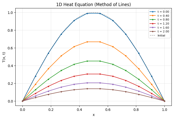
Max error at t=2.00 (vs exact PDE solution): 1.8522e-03
(Error includes spatial discretization from central differences)

9. Finite-Difference Discretization

For problems where high-order accuracy is not needed, finite differences offer a simpler alternative to collocation. The FDBuilder class provides the same high-level interface as DAEBuilder but uses finite-difference stencils (backward Euler, forward Euler, or central differences) instead of orthogonal collocation.

State variables have shape (nfe + 1,) — values at all grid points including both endpoints. Controls are piecewise constant per interval.

Let’s solve the same exponential decay \(dx/dt = -x\) using backward Euler and compare accuracy with the collocation approach.

nfe_values = [10, 20, 40]

fig, axes = plt.subplots(1, 2, figsize=(10, 4))

t_exact = np.linspace(0, 5, 200)
x_exact = np.exp(-t_exact)
axes[0].plot(t_exact, x_exact, "k-", linewidth=2, label="Exact")

colors = ["b", "r", "g"]

for nfe, color in zip(nfe_values, colors):
    # FDBuilder uses backward Euler by default
    m_fd = Model(f"fd_{nfe}")
    cs_fd = ContinuousSet("t", bounds=(0, 5), nfe=nfe)
    fd = FDBuilder(m_fd, cs_fd, method="backward")

    fd.add_state("x", initial=1.0, bounds=(0, 2))
    fd.set_ode(lambda t, states, alg, ctrl: {"x": -states["x"]})
    fd.discretize()
    m_fd.minimize(0)
    result_fd = m_fd.solve()

    t_fd, x_fd = fd.extract_solution(result_fd, "x")
    error_fd = np.abs(x_fd - np.exp(-t_fd))

    axes[0].plot(
        t_fd, x_fd, f"{color}o-", markersize=3, linewidth=1, label=f"Backward Euler (nfe={nfe})"
    )
    axes[1].semilogy(t_fd[1:], error_fd[1:], f"{color}o-", markersize=3, label=f"nfe={nfe}")

axes[0].set_xlabel("t")
axes[0].set_ylabel("x(t)")
axes[0].set_title("Finite Difference Solutions")
axes[0].legend(fontsize=8)
axes[0].grid(True, alpha=0.3)

axes[1].set_xlabel("t")
axes[1].set_ylabel("Absolute error")
axes[1].set_title("FD Error (Backward Euler)")
axes[1].legend(fontsize=8)
axes[1].grid(True, alpha=0.3)

plt.tight_layout()
plt.show()

# Compare FD vs collocation accuracy
print("\n=== Accuracy comparison (nfe=20) ===")

# Collocation with nfe=20, ncp=3
m_coll = Model("coll_compare")
cs_coll = ContinuousSet("t", bounds=(0, 5), nfe=20, ncp=3)
dae_coll = DAEBuilder(m_coll, cs_coll)
dae_coll.add_state("x", initial=1.0, bounds=(0, 2))
dae_coll.set_ode(lambda t, s, a, c: {"x": -s["x"]})
dae_coll.discretize()
m_coll.minimize(0)
r_coll = m_coll.solve()
t_c, x_c = dae_coll.extract_solution(r_coll, "x")
err_coll = np.max(np.abs(x_c - np.exp(-t_c)))

# FD with nfe=20
m_fd2 = Model("fd_compare")
cs_fd2 = ContinuousSet("t", bounds=(0, 5), nfe=20)
fd2 = FDBuilder(m_fd2, cs_fd2, method="backward")
fd2.add_state("x", initial=1.0, bounds=(0, 2))
fd2.set_ode(lambda t, s, a, c: {"x": -s["x"]})
fd2.discretize()
m_fd2.minimize(0)
r_fd2 = m_fd2.solve()
t_f, x_f = fd2.extract_solution(r_fd2, "x")
err_fd = np.max(np.abs(x_f - np.exp(-t_f)))

print(f"Collocation (nfe=20, ncp=3): max error = {err_coll:.2e}  ({20 * 4} variables)")
print(f"Backward Euler (nfe=20):     max error = {err_fd:.2e}  (21 variables)")
print("\nCollocation achieves much higher accuracy for similar problem size,")
print("but finite differences are simpler and work well for coarse approximations.")

=== Accuracy comparison (nfe=20) ===

Collocation (nfe=20, ncp=3): max error = 3.71e-06  (80 variables)
Backward Euler (nfe=20):     max error = 4.17e-02  (21 variables)

Collocation achieves much higher accuracy for similar problem size,
but finite differences are simpler and work well for coarse approximations.

Summary

The discopt.dae module provides two discretization approaches for dynamic optimization:

Feature	DAEBuilder (collocation)	FDBuilder (finite difference)
Accuracy	High-order (\(2n_{cp}-1\) for Radau)	First-order (Euler)
Algebraic variables	Yes (add_algebraic)	No
Second-order ODEs	Yes (add_second_order_state)	No
Integral objectives	Yes (dae.integral())	Manual summation
Least-squares fitting	Yes (dae.least_squares())	Yes (fd.least_squares())
Non-uniform elements	Yes (element_boundaries)	Yes (element_boundaries)
Problem size	Larger (more variables per element)	Smaller
Best for	High-accuracy, stiff systems, DAEs	Quick prototyping, simple ODEs

Key API methods:

• ContinuousSet(name, bounds, nfe, ncp, scheme, element_boundaries) — define the time domain

• align_time_grid(t_span, nfe, measurement_times) — snap element boundaries to measurement times

• add_state(name, initial, bounds, n_components) — differential states

• add_algebraic(name, bounds) — algebraic variables (DAEBuilder only)

• add_control(name, bounds) — piecewise-constant controls

• set_ode(rhs) — first-order ODE right-hand side

• set_algebraic(rhs) — algebraic equations

• set_second_order_ode(rhs) — acceleration for second-order ODEs

• discretize() — generate all variables and constraints

• least_squares(state_name, t_data, y_data) — sum-of-squared-residuals objective

• extract_solution(result, name) — extract time series from solve result

• integral(integrand) — quadrature-based integral expression

References

• Biegler [2010] – Nonlinear programming textbook with extensive coverage of collocation methods.

• Betts [2010] – Practical methods for optimal control using direct transcription.

• Cuthrell and Biegler [1987] – Original simultaneous collocation approach for DAE-constrained optimization.