Scaling ReLU Network Embeddings: discopt vs OMLT, and Depth vs Width

A trained ReLU network embedded in an optimization model becomes a mixed-integer linear program (MILP): every neuron whose pre-activation can take either sign gets one binary variable and four big-M constraints [Fischetti and Jo, 2018]. This notebook asks two practical questions about that encoding.

1. How does discopt scale against OMLT [Ceccon et al., 2022], the reference toolkit for this class, as the network grows? Both are run on the same networks, and both hand the MILP to HiGHS [Huangfu and Hall, 2018], which is discopt’s default backend for pure LP/MILP models.

2. At a fixed neuron budget, is it better to go wide or deep? The answer matters when you design a surrogate you intend to optimize over, not only predict with.

Everything below is measured, with the instrument named, and solve results are loaded from the CSV files committed next to this notebook rather than re-run here, so the numbers are exactly the ones discussed. The one live computation is the interval-bound analysis in the depth-vs-width section, which takes milliseconds. Commands to reproduce every table are at the end.

For the modeling API itself see Neural Network Embedding; for the strength of the big-M formulation and its alternatives see Anderson et al. [2020].

import json
from pathlib import Path

import matplotlib.pyplot as plt
import numpy as np
import pandas as pd

DATA = Path("data/relu_scaling")
sweep = pd.read_csv(DATA / "sweep_relu_bigm.csv")
split = pd.read_csv(DATA / "timing_split.csv")
slack = pd.read_csv(DATA / "slack_vs_native.csv")
dw = pd.read_csv(DATA / "depth_width.csv")
ARM = {"discopt": "discopt", "omlt+ref": "OMLT + HiGHS", "omlt+highs": "OMLT + HiGHS"}
print({k: len(v) for k, v in dict(sweep=sweep, split=split, slack=slack, depth_width=dw).items()})

{'sweep': 96, 'split': 84, 'slack': 354, 'depth_width': 45}

Setup and provenance

Networks	2 inputs in \([-1,1]^2\), \(L\) hidden ReLU layers of width \(w\), 1 linear output; weights \(\mathcal N(0, 1/\text{fan-in})\), biases \(\mathcal N(0, 0.1^2)\); objective: minimize the output
discopt	discopt.ml.add_predictor(..., method="relu_bigm") → default LP/MILP route → HiGHS
OMLT	OMLT 1.2.2 ReluBigMFormulation → Pyomo 6.10.1 SolverFactory("highs")
Solver	HiGHS 1.15.1 via highspy, identical options in both arms (only time_limit set)
Machine	4-core Intel Xeon @ 2.8 GHz; per-row load recorded where available
Code	sweep: main at e1a5388; timing split, slack experiment, depth vs width: main at b7178ea

Two caveats apply throughout. The weights are random, not trained: random networks have almost no stable neurons, so they are close to the hardest case for a given size. And there are only 2 inputs, so the networks are small in input dimension and large only in their hidden layers.

1. Model size: the two encodings are the same size

Both encodings add one binary per unstable hidden neuron. discopt’s relu_bigm formulation uses the interval bounds to drop the binary for any neuron that is provably always on or always off, which is why it occasionally has one binary fewer.

size = (sweep.query("seed == 0 and arm in ['discopt', 'omlt+ref']")
        .pivot_table(index=["depth", "width"], columns="arm", values=["vars", "bins"])
        .astype(int))
size.columns = [f"{v} ({ARM[a]})" for v, a in size.columns]
size

		bins (discopt)	bins (OMLT + HiGHS)	vars (discopt)	vars (OMLT + HiGHS)
depth	width
1	10	9	10	34	40
	25	25	25	80	85
	50	50	50	155	160
	100	99	100	304	310
2	10	19	20	64	70
	25	50	50	155	160
	50	100	100	305	310
	100	199	200	604	610
3	10	29	30	94	100
	25	75	75	230	235
	50	150	150	455	460
	100	299	300	904	910

2. Scaling: same instances solved, same answers

Each instance was solved by both tools with a 30 s limit, two seeds per size.

cert = (sweep[sweep.arm.isin(["discopt", "omlt+ref"])]
        .groupby(["depth", "width", "arm"]).cert.sum().unstack("arm").astype(int))
cert.columns = [f"certified, {ARM[a]} (of 2)" for a in cert.columns]
both = sweep.pivot_table(index=["depth", "width", "seed"], columns="arm", values="objective")
agree = both.dropna(subset=["discopt", "omlt+ref"])
print("certified objectives that disagree by more than 1e-6:",
      int((abs(agree["discopt"] - agree["omlt+ref"]) > 1e-6).sum()), "of", len(agree))
cert

certified objectives that disagree by more than 1e-6: 0 of 14

		certified, discopt (of 2)	certified, OMLT + HiGHS (of 2)
depth	width
1	10	2	2
	25	2	2
	50	2	2
	100	2	2
2	10	2	2
	25	2	2
	50	0	0
	100	0	0
3	10	2	2
	25	0	0
	50	0	0
	100	0	0

fig, axes = plt.subplots(1, 2, figsize=(11, 4.2))
ok = sweep[sweep.cert == 1].pivot_table(index=["depth", "width", "seed"], columns="arm", values="wall")
ok = ok.dropna(subset=["discopt", "omlt+ref"])
ax = axes[0]
for d, mk in zip((1, 2, 3), "os^"):
    sub = ok.xs(d, level="depth")
    ax.scatter(sub["omlt+ref"], sub["discopt"], marker=mk, label=f"depth {d}")
lim = [0.01, 60]
ax.plot(lim, lim, "k--", lw=0.8, label="equal time")
ax.set(xscale="log", yscale="log", xlim=lim, ylim=lim,
       xlabel="OMLT + HiGHS wall (s)", ylabel="discopt wall (s)",
       title="Certified instances, one run each")
ax.legend()

ax = axes[1]
for arm, mk in (("discopt", "o"), ("omlt+ref", "s")):
    g = sweep[(sweep.arm == arm) & (sweep.cert == 1)].groupby(["depth", "width"]).wall.median()
    for d in (1, 2, 3):
        if d in g.index.get_level_values(0):
            s = g.xs(d)
            ax.plot(s.index, s.values, marker=mk, ls="-" if arm == "discopt" else ":",
                    label=f"{ARM[arm]}, depth {d}")
ax.set(xscale="log", yscale="log", xlabel="hidden width", ylabel="median wall, certified (s)",
       title="Time to certify vs width")
ax.legend(fontsize=7)
fig.tight_layout()

On the instances that neither tool certified, compare what each had found. The sweep also ran SCIP on discopt’s model (discopt+scip), which is shown here only for this comparison.

unc = sweep.groupby(["width", "depth", "seed"]).filter(
    lambda g: not g[g.arm.isin(["discopt", "omlt+ref"])].cert.any())
inc = (unc.assign(has_incumbent=unc.objective.notna())
          .groupby("arm").agg(instances=("has_incumbent", "size"),
                              with_incumbent=("has_incumbent", "sum")))
inc.index = [{"discopt+scip": "SCIP (on discopt's model)", "omlt+discopt": "discopt (on OMLT's model)"}
             .get(a, ARM.get(a, a)) for a in inc.index]
inc

	instances	with_incumbent
discopt	10	0
SCIP (on discopt's model)	10	10
discopt (on OMLT's model)	10	0
OMLT + HiGHS	10	0

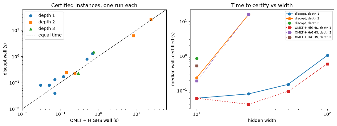
Reading. Both tools certify exactly the same instances at every size, and every certified objective agrees. Both stop certifying within 30 s at the same point — depth 2 at width 50, depth 3 at width 25 — while every depth-1 network up to width 100 solves in about a second. Model size alone does not set the difficulty: 100×1 (99 binaries) solves in about a second, while 25×3 (75 binaries) does not finish.

These are single runs, so the scatter in the left panel mixes real differences with run-to-run noise. The next section repeats a subset to separate the two.

3. Where the time goes (repeated, interleaved)

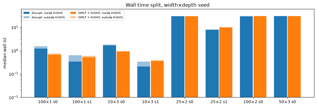
Each solve ran in a fresh process after an untimed warm-up solve (so imports and first-call setup are excluded), the two tools alternated, and every highspy.Highs.run call was timed. Overhead is wall time outside HiGHS: model extraction, translation, and in discopt’s case the certificate checks.

split["total"] = split["build"] + split["solve"]
split["overhead"] = split["solve"] - split["highs"]
g = split.groupby(["spec", "arm"])
summary = pd.DataFrame({
    "n": g.size(),
    "total median (s)": g.total.median(),
    "total sd (s)": g.total.std(),
    "overhead median (s)": g.overhead.median(),
    "HiGHS median (s)": g.highs.median(),
    "HiGHS calls": g.highs_calls.median().astype(int),
}).round(3)
summary.index = summary.index.set_levels([summary.index.levels[0], [ARM[a] for a in summary.index.levels[1]]])
summary

		n	total median (s)	total sd (s)	overhead median (s)	HiGHS median (s)	HiGHS calls
spec	arm
100:1:0	discopt	6	1.565	0.232	0.294	1.223	5
	OMLT + HiGHS	6	0.748	0.061	0.058	0.662	1
100:1:1	discopt	6	0.627	0.019	0.270	0.339	5
	OMLT + HiGHS	6	0.589	0.037	0.053	0.518	1
100:2:0	discopt	3	30.238	0.159	0.966	29.177	1
	OMLT + HiGHS	3	30.346	0.034	0.133	30.012	1
10:3:0	discopt	6	1.790	0.047	0.115	1.671	5
	OMLT + HiGHS	6	0.954	0.027	0.023	0.919	1
10:3:1	discopt	6	0.334	0.008	0.120	0.207	5
	OMLT + HiGHS	6	0.393	0.009	0.022	0.358	1
25:2:0	discopt	6	30.031	0.011	0.157	29.872	2
	OMLT + HiGHS	6	29.856	0.519	0.033	29.802	1
25:2:1	discopt	6	7.967	0.226	0.170	7.762	5
	OMLT + HiGHS	6	9.931	0.389	0.033	9.861	1
50:3:0	discopt	3	30.199	0.013	0.609	29.556	1
	OMLT + HiGHS	3	30.186	0.012	0.093	30.007	1

specs = list(dict.fromkeys(split.spec))
fig, ax = plt.subplots(figsize=(11, 3.8))
x = np.arange(len(specs))
for k, (arm, off) in enumerate((("discopt", -0.2), ("omlt+highs", 0.2))):
    s = split[split.arm == arm].groupby("spec")
    hi = s.highs.median().reindex(specs)
    ov = (s.overhead.median() + s.build.median()).reindex(specs)
    ax.bar(x + off, hi, 0.38, label=f"{ARM[arm]}: inside HiGHS", color=f"C{k}")
    ax.bar(x + off, ov, 0.38, bottom=hi, label=f"{ARM[arm]}: outside HiGHS", color=f"C{k}", alpha=0.45)
ax.set_xticks(x, [s.replace(":", "×", 1).replace(":", " s") for s in specs])
ax.set(yscale="log", ylim=(0.01, 60), ylabel="median wall (s)",
       title="Wall time split, width×depth seed")
ax.legend(fontsize=7, ncol=2)
fig.tight_layout()

Reading.

• discopt has a fixed overhead of roughly 0.1–0.3 s per solve outside HiGHS (Pyomo: 0.02–0.06 s). It is extraction, the standard form, and the certificate work — discopt does not take HiGHS’s word for the answer; it re-verifies the incumbent and cross-checks the bound with extra LP solves. Those extra Highs.run calls (the 5 vs 1 in the table) are not where the time goes: instrumented on 10×3 seed 0 they cost 7 ms of a 1.87 s solve (recorded in docs/dev/lp-milp-highs-routing-plan.md §12), so the overhead is mostly Python-side.

• Inside HiGHS the time goes both ways. discopt is faster on some instances and slower on others. MIP search is chaotic: two algebraically equivalent models routinely take different branch-and-bound paths.

• At the time limit OMLT’s final dual bound is tighter on 50×3 (−13.06 vs −13.75), identically on every repeat. discopt’s overhead there is about 0.6 s of 30 s, so this is the model and search path, not lost time budget.

4. Why discopt can be slower: the standard form

discopt’s LP/MILP route hands HiGHS the model in standard form, \(\min c^\top x\) s.t. \(Ax=b,\ \ell\le x\le u\), with one slack column per inequality row. That is deliberate. discopt certifies every LP answer itself, and its certificates — a rigorous lower bound from HiGHS’s duals, infeasibility rays, a phase-1 proof — are all stated for that form. Solving exactly the form being verified means HiGHS’s duals and rays refer to the very rows and columns that are checked, with no translation layer to get wrong. For an LP that is the right trade.

For a MILP it costs: the branch-and-cut sees about twice as many columns (10×3: 210 vs OMLT’s 100). The MILP’s certificate does not depend on the slack columns, so an experiment folded each slack back into its row’s bounds — the same model, minus the slack columns — and timed HiGHS on both forms (issue #1600).

fin = slack.groupby(["name", "form"]).agg(wall=("wall", "median"), status=("status", "first")).unstack("form")
fin = fin[(fin["status"]["std"] == "Optimal") & (fin["status"]["native"] == "Optimal")]
fin = pd.DataFrame({"std": fin["wall"]["std"], "native": fin["wall"]["native"]})
def family(n):
    if n.startswith("relu"):
        return "ReLU depth " + n.split("x")[1][0]
    return {"mknap": "knapsack", "cfl": "facility location", "setcover": "set cover",
            "lotsize": "lot sizing"}[n.split("_")[0]]
fin["family"] = [family(n) for n in fin.index]
fin["ratio"] = fin["native"] / fin["std"]
tab = fin.groupby("family").agg(
    n=("ratio", "size"),
    geomean_ratio=("ratio", lambda r: float(np.exp(np.log(r).mean()))),
    native_faster=("ratio", lambda r: int((r < 1).sum())),
    total_std_s=("std", "sum"), total_native_s=("native", "sum"))
tab["total_ratio"] = tab.total_native_s / tab.total_std_s
print(f"{len(fin)} instances: median ratio {fin.ratio.median():.3f}, native faster on "
      f"{int((fin.ratio < 1).sum())}/{len(fin)}, total {fin['std'].sum():.1f} s -> {fin['native'].sum():.1f} s")
tab.sort_values("total_ratio").round(3)

59 instances: median ratio 0.805, native faster on 37/59, total 168.6 s -> 112.1 s

	n	geomean_ratio	native_faster	total_std_s	total_native_s	total_ratio
family
set cover	6	0.540	6	76.747	41.603	0.542
facility location	6	0.691	5	1.896	1.046	0.552
ReLU depth 2	10	0.909	6	63.518	44.862	0.706
ReLU depth 1	20	0.936	11	6.167	4.756	0.771
knapsack	6	0.815	4	12.602	11.449	0.909
lot sizing	6	1.043	3	1.042	1.035	0.993
ReLU depth 3	5	1.303	2	6.672	7.383	1.107

Without the slack columns HiGHS is faster in aggregate — total time down about a third — with the gain concentrated on the larger, harder models (set cover, facility location, depth-2 networks). Instance by instance it is noisy, for the same search-path reason as above. The route is deliberately not changed (#1600, closed as not planned): certification is already at parity, the gain is wall time only and inconsistent per instance, and it would put a second model representation on a route whose rule is that what HiGHS solves is exactly what discopt verifies. It would be revisited if MILP wall time became a priority or a broad MILP panel showed a consistent win.

In short: at equal model size discopt is at parity with OMLT on which instances it solves and what answer it returns. It pays a small fixed cost for verifying the answer, and a variable cost for the standard form, which is kept on purpose.

5. Depth vs width

Hold the number of hidden neurons fixed and vary how they are arranged: 60 neurons as 60×1, 30×2, 20×3, 15×4, 12×5 or 10×6. The number of binaries barely changes — nearly every neuron of a random network is unstable — so if difficulty tracked the binary count, all arrangements would be equally hard.

The mechanism: bounds loosen layer by layer

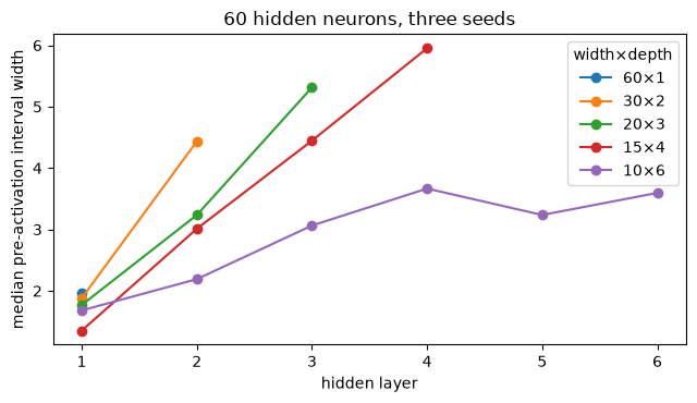
The big-M constants come from interval bounds on each neuron’s pre-activation, propagated layer by layer from the input box (discopt.ml.bounds.propagate_bounds, the same routine the formulation uses). Interval arithmetic cannot see correlations between neurons, so every layer widens the intervals of the next. Deeper layers get looser bounds, larger big-M constants, and a weaker LP relaxation.

from discopt.ml.bounds import propagate_bounds
from discopt.ml.network import DenseLayer, NetworkDefinition


def make_net(d, width, depth, act, seed):
    # identical to discopt_benchmarks/scripts/omlt_scaling_panel.py::make_net
    rng = np.random.default_rng(seed)
    sizes = [d] + [width] * depth + [1]
    return [(rng.normal(0, 1 / np.sqrt(a), size=(a, b)), rng.normal(0, 0.1, size=b),
             act if i < depth else "linear")
            for i, (a, b) in enumerate(zip(sizes[:-1], sizes[1:], strict=True))]


def layer_bounds(budget, depth, seed=0, box=1.0):
    layers = make_net(2, budget // depth, depth, "relu", seed)
    net = NetworkDefinition([DenseLayer(w, b, a) for w, b, a in layers],
                            input_bounds=(np.full(2, -box), np.full(2, box)))
    out = []
    for k, lb in enumerate(propagate_bounds(net)[:-1]):
        lo, hi = np.asarray(lb.pre_lb), np.asarray(lb.pre_ub)
        out.append(dict(layer=k + 1, median_width=float(np.median(hi - lo)),
                        unstable=int(((lo < 0) & (hi > 0)).sum()), neurons=len(lo)))
    return pd.DataFrame(out)


fig, ax = plt.subplots(figsize=(6.5, 3.8))
for depth in (1, 2, 3, 4, 6):
    t = pd.concat([layer_bounds(60, depth, s) for s in range(3)]).groupby("layer").median_width.median()
    ax.plot(t.index, t.values, marker="o", label=f"{60 // depth}×{depth}")
ax.set(xlabel="hidden layer", ylabel="median pre-activation interval width",
       title="60 hidden neurons, three seeds")
ax.legend(title="width×depth")
fig.tight_layout()
pd.concat({f"{60 // d}x{d}": layer_bounds(60, d).set_index("layer") for d in (1, 2, 3, 6)})

		median_width	unstable	neurons
	layer
60x1	1	1.986236	59	60
30x2	1	1.881663	30	30
	2	4.435060	30	30
20x3	1	1.770387	20	20
	2	3.152288	20	20
	3	4.934005	20	20
10x6	1	1.682028	9	10
	2	2.441509	10	10
	3	3.064234	10	10
	4	3.666400	10	10
	5	3.236683	10	10
	6	3.595465	10	10

The consequence: solve time at a fixed neuron budget

Hidden-neuron budgets of 60 and 120, depths 1–6, three seeds, 60 s limit, solved by discopt with its default route. A timed-out solve is plotted at the limit.

wide = dw[dw.box == 1.0]
fig, axes = plt.subplots(1, 2, figsize=(11, 4))
for k, (budget, mk) in enumerate(((60, "o"), (120, "s"))):
    s = wide[wide.budget == budget]
    axes[0].scatter(s.depth + (0.08 if budget == 120 else -0.08), s.wall, marker=mk,
                    label=f"{budget} neurons", alpha=0.8, color=f"C{k}")
    med = s.groupby("depth").wall.median()
    axes[0].plot(med.index, med.values, ls=":", color=f"C{k}")
    c = s.groupby("depth").cert.sum()
    axes[1].bar(c.index + (0.2 if budget == 120 else -0.2), c.values, 0.4,
                label=f"{budget} neurons", color=f"C{k}")
axes[0].axhline(60, color="k", lw=0.8, ls="--")
axes[0].set(yscale="log", xlabel="depth (width = budget / depth)", ylabel="wall (s)",
            title="Time to certify (limit 60 s, dashed)")
axes[1].set(xlabel="depth", ylabel="seeds certified (of 3)", ylim=(0, 3.2),
            title="Certified within 60 s")
for ax in axes:
    ax.legend()
fig.tight_layout()
(wide.groupby(["budget", "depth"])
     .agg(width=("width", "first"), binaries=("binaries", "median"),
          certified=("cert", "sum"), seeds=("cert", "size"),
          median_wall_s=("wall", "median"), median_big_M=("big_m", "median"))
     .round(2))

		width	binaries	certified	seeds	median_wall_s	median_big_M
budget	depth
60	1	60	60.0	3	3	0.45	2.71
	2	30	60.0	3	3	15.19	4.88
	3	20	60.0	2	3	48.75	5.25
	4	15	60.0	0	3	60.01	5.73
	5	12	60.0	1	3	60.01	4.43
	6	10	60.0	1	3	60.02	4.35
120	1	120	120.0	3	3	2.09	3.19
	2	60	120.0	0	3	60.02	5.04
	3	40	120.0	0	3	60.02	11.15
	4	30	120.0	0	3	60.03	16.34
	5	24	120.0	0	3	60.02	22.68
	6	20	120.0	0	3	60.02	24.74

Input bounds

The same networks with the input box narrowed from \([-1,1]^2\) to \([-0.25,0.25]^2\). Narrower inputs shrink every interval downstream, which stabilizes neurons (fewer binaries) and shrinks the big-M constants.

nar = dw[dw.box < 1.0][["budget", "depth", "seed"]].drop_duplicates()
cmp = dw.merge(nar, on=["budget", "depth", "seed"])
(cmp.pivot_table(index=["budget", "depth", "seed"], columns="box",
                 values=["binaries", "big_m", "wall", "cert"])
    .round(2))

			big_m		binaries		cert		wall
		box	0.25	1.00	0.25	1.00	0.25	1.00	0.25	1.00
budget	depth	seed
60	3	0	1.38	4.29	57.0	60.0	1.0	1.0	10.06	48.75
		1	1.37	5.25	59.0	60.0	1.0	0.0	34.02	60.02
		2	1.51	5.69	56.0	60.0	1.0	1.0	12.32	44.48
	4	0	1.61	5.71	57.0	60.0	1.0	0.0	6.27	60.04
		1	1.60	5.73	54.0	59.0	1.0	0.0	9.65	60.01
		2	1.82	7.24	59.0	60.0	1.0	0.0	43.41	60.01
120	3	0	3.12	12.00	118.0	120.0	0.0	0.0	60.05	60.02
		1	2.76	11.15	115.0	119.0	0.0	0.0	60.02	60.03
		2	2.77	10.78	118.0	120.0	0.0	0.0	60.02	60.02

Reading

• Same binaries, very different difficulty. At 60 neurons every arrangement has 59–60 binaries, yet 60×1 certifies in under a second, 30×2 in about 15 s, 20×3 in about 50 s (two seeds of three), and from depth 4 on nearly nothing certifies within 60 s. At 120 neurons only the single-layer network certifies (about 2 s); every deeper arrangement times out.

• The big-M constants track the bound loosening. At 120 neurons the median largest big-M grows from 3.2 (one layer) to 11 (three layers) and 25 (six layers), exactly the layer-by-layer widening shown above.

• Beyond depth 3 the trend is not perfectly monotone at the 60-neuron budget (depths 5 and 6 each certify one seed of three; depth 4 none). That is consistent with the mechanism plot, where very narrow layers widen the intervals less per layer, but three seeds cannot settle it. All three depths are far harder than one or two layers.

• Input bounds matter a lot. Narrowing the input box from \(\pm 1\) to \(\pm 0.25\) stabilized only a few neurons (59–60 → 54–59 binaries) but shrank the big-M constants 3–4× (per seed, 3.1× to 4.0×), and took the 60-neuron depth-3 and depth-4 networks from 2 of 6 certified to 6 of 6. It was not enough for 120×3.

6. Best practices for optimizing over a ReLU network

Each recommendation is tied to the evidence above or to the literature.

1. Prefer wide and shallow when you have a choice. At a fixed neuron budget the binary count is the same, but every extra layer loosens the big-M bounds of all the layers after it (Section 5). If a shallower network fits your data nearly as well, it is far cheaper to optimize over. Deeper networks can represent more linear regions per neuron [Serra et al., 2018] — that is the expressivity you pay for.

2. Bound the inputs as tightly as the application allows. The input box is the seed of every big-M constant. Narrowing it stabilizes neurons (they lose their binaries entirely) and shrinks the remaining constants (Section 5). Declare tight bounds on the input variables, or pass input_bounds= to add_predictor.

3. Stable neurons are free; train for them. A neuron that is provably always on or always off needs no binary, and discopt drops it automatically (Section 1). Regularizers that push pre-activations away from zero make far more neurons stable and the MILP correspondingly smaller [Xiao et al., 2019]; tighter per-neuron bounds have the same effect [Tjeng et al., 2019].

4. Expect difficulty to grow with depth, not just size. In the sweep, every depth-1 network up to 100 neurons certified in about a second; depth 2 ran out of time at 100 neurons and depth 3 at 75 (Section 2). Budget time accordingly.

5. For a solution fast, not a proof, watch the incumbent. On the networks neither tool certified in 30 s, HiGHS (and therefore discopt and OMLT+HiGHS) had not found any feasible point, while SCIP found one on every such instance in the same benchmark (Section 2’s sweep, SCIP arm). If you need a good point quickly on a large network, supply an initial point (for example the network evaluated at a sensible input) or use a solver with stronger primal heuristics.

6. Use ReLU, not smooth activations, if you intend to certify. The ReLU embedding is a MILP that discopt and OMLT solve equally well. Smooth activations (sigmoid, tanh) become nonconvex nonlinear programs, which are much harder to certify. In the same benchmark run (at e1a5388, sigmoid full-space, same grid of sizes) discopt certified 0 of 24 networks against 20 of 24 for OMLT with SCIP. Those numbers predate array-row bound propagation (#1568, since made the default), which was aimed at exactly this gap; they are not reproduced here and should be re-measured before being relied on.

7. Caveats

• Random networks, not trained ones. Trained networks typically have many more stable neurons and are easier at the same size.

• Two inputs only; one machine; a single solver backend (HiGHS) for the MILP.

• The scaling sweep is one run per instance; Section 3’s repeats are the timing evidence.

8. Reproduce

The scripts live in discopt_benchmarks/scripts/:

# Section 2 (both tools, sizes x seeds; --forms relu:bigm for this notebook)
python -u omlt_scaling_panel.py --forms relu:bigm --out sweep.tsv
# Section 3 (repeated, interleaved, with the HiGHS-time split)
python -u relu_timing_split.py --reps 6 --tl 30 --out timing_split.tsv
# Section 4 (slack vs native rows)
python -u milp_slack_vs_native_rows.py --tl 60 --reps 3 --out slack_vs_native.tsv
# Section 5 (depth vs width)
python -u relu_depth_width.py --tl 60 --out depth_width.tsv

The CSV files in docs/notebooks/data/relu_scaling/ are those outputs.