
Hybrid physics + ML: training neural DAEs#
Many models are part physics, part data: a set of conservation laws or a dynamic (ODE/DAE) model in which one term — a reaction rate, a transport coefficient, a closure — is unknown and must be learned from data. This notebook shows how to train such a hybrid model in discopt using the simultaneous approach of Lueg et al. [2025]: discretize the dynamics with orthogonal collocation, make the neural-network weights and the discretized states joint decision variables, and solve the whole thing as one sparse nonlinear program.
Unlike the classic neural-ODE approach [Chen et al., 2018], which differentiates through an ODE integrator at every training step, the simultaneous approach [Biegler, 2010] never calls an integrator: the collocation equations enforce the dynamics as algebraic constraints, and a single NLP solve fits the weights and reconstructs the state trajectory at once.
discopt gives you two halves of one story:
Train a surrogate whose weights are decision variables (
discopt.ml.TrainableNetwork/TrainableKernelExpansion) — this notebook.Freeze the trained surrogate into the frozen-embedding path (
discopt.ml.add_predictor, following OMLT [Ceccon et al., 2022] and [Anderson et al., 2020]) and optimize over it with global guarantees [Schweidtmann and Mitsos, 2019] — the last section closes this loop.
A batch-reactor problem#
Consider an isothermal batch reactor \(A \to B\) whose true kinetics are unknown to us:
with a Michaelis–Menten-like true rate \(r(c) = 1.5\,c^2 / (0.3 + c)\). We observe noisy concentrations of both species and want to learn \(r\) while reconstructing the trajectories. The physics (the stoichiometric mass balances) is known; only the rate law is replaced by a trainable surrogate.
import numpy as np
from scipy.integrate import solve_ivp

CA0, CB0, TF = 1.0, 0.0, 2.0
NOISE = 0.01


def r_true(c):
    return 1.5 * c**2 / (0.3 + c)


def make_data(seed, ca0=CA0, n_obs=15):
    rng = np.random.default_rng(seed)
    t = np.linspace(0.05, TF, n_obs)
    sol = solve_ivp(lambda t, y: [-r_true(y[0]), r_true(y[0])],
                    (0, TF), [ca0, CB0], t_eval=t, rtol=1e-10, atol=1e-12)
    yA = sol.y[0] + NOISE * rng.standard_normal(n_obs)
    yB = sol.y[1] + NOISE * rng.standard_normal(n_obs)
    return t, yA, yB


t_data, yA, yB = make_data(seed=0)
print(f"{len(t_data)} noisy observations of cA and cB on [0, {TF}]")
15 noisy observations of cA and cB on [0, 2.0]
Build the hybrid model#
We replace the unknown rate law with a small feedforward network
(TrainableNetwork) whose weights are decision variables. The dynamics are
transcribed with orthogonal collocation on finite elements via
discopt.dae.DAEBuilder; the network is simply called inside the ODE right-hand
side, so its weights enter the collocation constraints directly.
We use a smooth activation (tanh here, softplus is the other common
choice) — a gradient-based NLP solver cannot handle ReLU’s kink, so the
trainable path refuses it.
import discopt.modeling as dm
from discopt.dae import ContinuousSet, DAEBuilder
from discopt.ml import TrainableNetwork

m = dm.Model("neural_dae")
net = TrainableNetwork(m, sizes=[1, 6, 1], activation="tanh",
                       weight_bounds=(-8.0, 8.0), name="rate")

cs = ContinuousSet("t", (0.0, TF), nfe=20, ncp=2, scheme="radau")
dae = DAEBuilder(m, cs)
dae.add_state("cA", bounds=(0.0, 1.5), initial=CA0)
dae.add_state("cB", bounds=(0.0, 1.5), initial=CB0)


def rhs(t, s, a, u):
    r = net(s["cA"])           # expression in, expression out
    return {"cA": -r, "cB": r}


dae.set_ode(rhs)
dvars = dae.discretize()
print(f"{net.n_parameters()} network weights + "
      f"{sum(v.size for v in m._variables) - net.n_parameters()} collocation states")
19 network weights + 120 collocation states
Objective and warm start#
The training objective is a least-squares data mismatch (evaluated by exact collocation-polynomial interpolation at the measurement times) plus a small \(L_2\) weight penalty. We warm-start the states by interpolating the noisy data onto the collocation grid, and the weights with a Glorot-style random draw.
lsq = dae.least_squares("cA", t_data, yA) + dae.least_squares("cB", t_data, yB)
m.minimize(lsq + 1e-4 * net.l2_penalty())

tp = dae._element_points()
cA_init = np.interp(tp, np.concatenate([[0], t_data]), np.concatenate([[CA0], yA]))
cB_init = np.interp(tp, np.concatenate([[0], t_data]), np.concatenate([[CB0], yB]))
warm = {dvars["cA"]: cA_init, dvars["cB"]: cB_init} | net.initial_values(seed=0)
Train#
discopt.ml.train is a thin wrapper around a single local NLP solve: it
builds the evaluator (with the Gauss-Newton Hessian approximation, which is exact
for a least-squares objective whose residuals are linear in the states) and calls
the in-house interior-point backend. Because it is a local solve, the result
carries no global optimality certificate — the last section shows how to obtain
one for a frozen surrogate.
from discopt.ml import train

result = train(m, initial_solution=warm, options={"max_iter": 3000, "tol": 1e-8})
print(f"status = {result.status.name}, iterations = {result.iterations}, "
      f"objective = {result.objective:.3e}")
status = OPTIMAL, iterations = 15, objective = 2.199e-03
How the training actually works#
There is no stochastic gradient descent here — no minibatches, no learning rate,
no epochs. train assembles a single constrained nonlinear program and hands
it to a second-order interior-point solver. The steps:
The surrogate emits equations, not numbers.
net(s["cA"])builds a symbolic expression graph whose leaves include the weight variables. Nothing is evaluated yet.The dynamics become hard equality constraints.
discretize()turns the ODE into the collocation equations \(\sum_k A_{jk}\,x_{ik} = h_i\,f(x_{ij})\) at every finite element \(i\) and collocation point \(j\) — with the unknown \(f\) being the surrogate. The physics is enforced as equations, not integrated.One flat decision vector. The NN weights and every discretized state are optimized together; the data mismatch is the objective.
Derivatives come from JAX autodiff over the graph — the objective gradient, the constraint Jacobian, and either the exact Lagrangian Hessian or (the default for a sum-of-squares objective) the Gauss-Newton approximation \(2J^\top J\). Nothing is hand-coded.
POUNCE (an interior-point method) solves it by repeatedly forming and factorizing the KKT system and taking Newton steps to first-order optimality.
Because the states are decision variables too, each Newton step nudges the weights and re-solves the discretized dynamics through the KKT linear system — so there is no inner ODE solve and no adjoint. That coupling is why this converges in ~15–20 iterations instead of thousands of SGD steps (Biegler’s simultaneous approach).
Sparsity is automatic. The evaluator detects the sparsity pattern of the expression DAG and reports the true nonzero positions of the Jacobian and Hessian to the solver, so POUNCE factorizes a sparse KKT system — essential, because a collocation problem is block-bordered: each constraint touches only the states in its element plus the shared weights. Below we inspect the assembled problem: the Jacobian is ~10 % dense even for this tiny model, and the density falls as the horizon grows. (For value computation the evaluator switches to a compressed coloring scheme above ~50 variables and <15 % density; smaller/denser problems evaluate densely but still hand the solver the sparse structure.)
from discopt._relax.nlp_evaluator import NLPEvaluator

ev = NLPEvaluator(m, gauss_newton=True)   # the same evaluator train() builds
n_w = net.n_parameters()
rows, cols = ev.jacobian_structure()      # COO nonzero positions handed to POUNCE
nnz, size = len(rows), ev.n_constraints * ev.n_variables

print(f"decision variables  : {ev.n_variables}  "
      f"({n_w} NN weights + {ev.n_variables - n_w} collocation states)")
print(f"equality constraints : {ev.n_constraints}  (collocation + continuity + ICs)")
print(f"constraint Jacobian  : {nnz} nonzeros / {size}  = {100 * nnz / size:.1f}% dense")
print(f"sparse structure used: {ev.has_sparse_structure()}")
print(f"Gauss-Newton Hessian : {ev.is_gauss_newton}")
decision variables  : 139  (19 NN weights + 120 collocation states)
equality constraints : 118  (collocation + continuity + ICs)
constraint Jacobian  : 1876 nonzeros / 16402  = 11.4% dense
sparse structure used: True
Gauss-Newton Hessian : True
Assess honestly#
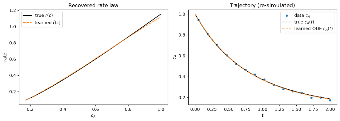
Two checks. First, does the learned rate law match the truth over the range the data visited? Second — the honest generalization test — if we take the learned rate law and integrate the ODE from scratch with a standard solver, do we recover the true trajectory? The assessment code lives here in the notebook, not in the library.
frozen = net.freeze(result)   # NetworkDefinition; forward() matches the trained net


def r_hat(c):
    return frozen.forward(np.atleast_1d(c).reshape(-1, 1)).ravel()


c_grid = np.linspace(float(yA.min()), CA0, 100)
rate_rmse = float(np.sqrt(np.mean((r_hat(c_grid) - r_true(c_grid)) ** 2)))

truth = solve_ivp(lambda t, y: [-r_true(y[0]), r_true(y[0])],
                  (0, TF), [CA0, CB0], t_eval=np.linspace(0, TF, 50),
                  rtol=1e-10, atol=1e-12)
learned = solve_ivp(lambda t, y: [-float(r_hat(y[0])[0]), float(r_hat(y[0])[0])],
                    (0, TF), [CA0, CB0], t_eval=truth.t, rtol=1e-9, atol=1e-11)
resim_rmse = float(np.sqrt(np.mean((learned.y[0] - truth.y[0]) ** 2)))

print(f"rate-law RMSE over visited range: {rate_rmse:.4f}")
print(f"re-simulation RMSE vs truth:      {resim_rmse:.4f}  (noise level {NOISE})")
rate-law RMSE over visited range: 0.0107
re-simulation RMSE vs truth:      0.0025  (noise level 0.01)
import matplotlib.pyplot as plt

fig, (ax1, ax2) = plt.subplots(1, 2, figsize=(11, 4))

ax1.plot(c_grid, r_true(c_grid), "k-", label="true $r(c)$")
ax1.plot(c_grid, r_hat(c_grid), "C1--", label="learned $\\hat r(c)$")
ax1.set_xlabel("$c_A$"); ax1.set_ylabel("rate"); ax1.set_title("Recovered rate law")
ax1.legend()

ax2.plot(t_data, yA, "C0o", ms=4, label="data $c_A$")
ax2.plot(truth.t, truth.y[0], "k-", label="true $c_A(t)$")
ax2.plot(learned.t, learned.y[0], "C1--", label="learned-ODE $c_A(t)$")
ax2.set_xlabel("t"); ax2.set_ylabel("$c_A$"); ax2.set_title("Trajectory (re-simulated)")
ax2.legend()
fig.tight_layout()
A kernel surrogate: linear in its parameters#
A neural network is not the only choice. A kernel / Gaussian-process-mean expansion \(r(x) = \sum_j \alpha_j\, k(x, c_j)\) with fixed centers and lengthscale is linear in its trainable coefficients \(\alpha\). That makes the ML block add no nonconvexity of its own: zero initialization suffices, there are no weight-symmetry local minima, and conditioning is excellent. The hyperparameters (centers, lengthscale) stay outside the NLP — tune them with a separate marginal-likelihood or cross-validation loop.
from discopt.ml import TrainableKernelExpansion

m3 = dm.Model("kernel_dae")
ke = TrainableKernelExpansion(m3, centers=np.linspace(0.0, 1.05, 12),
                              lengthscale=0.12, name="rate")

cs3 = ContinuousSet("t", (0.0, TF), nfe=20, ncp=2, scheme="radau")
dae3 = DAEBuilder(m3, cs3)
dae3.add_state("cA", bounds=(0.0, 1.5), initial=CA0)
dae3.add_state("cB", bounds=(0.0, 1.5), initial=CB0)
dae3.set_ode(lambda t, s, a, u: {"cA": -ke(s["cA"]), "cB": ke(s["cA"])})
dv3 = dae3.discretize()
m3.minimize(dae3.least_squares("cA", t_data, yA) + dae3.least_squares("cB", t_data, yB)
            + 1e-4 * ke.l2_penalty())

tp3 = dae3._element_points()
warm3 = {
    dv3["cA"]: np.interp(tp3, np.concatenate([[0], t_data]), np.concatenate([[CA0], yA])),
    dv3["cB"]: np.interp(tp3, np.concatenate([[0], t_data]), np.concatenate([[CB0], yB])),
} | ke.initial_values()
res3 = train(m3, initial_solution=warm3, options={"max_iter": 3000, "tol": 1e-8})
print(f"kernel surrogate ({ke.n_parameters()} coefficients, zero init): "
      f"{res3.status.name} in {res3.iterations} iterations")
kernel surrogate (12 coefficients, zero init): OPTIMAL in 12 iterations
Closing the loop: train, then freeze, then optimize#
The trained surrogate bridges back to the frozen embedding path. Once frozen
into a NetworkDefinition, the network can be embedded in a design or control
optimization and solved with discopt’s global machinery
[Schweidtmann and Mitsos, 2019] — the two halves of discopt.ml become one workflow.
Here we simply ask: over the operating range, at what \(c_A\) is the (learned) rate
maximized?
design = dm.Model("use_frozen_rate")
from discopt.ml import add_predictor

c_in = design.continuous("cA", shape=(1,), lb=0.05, ub=1.0)
rate_out, _formulation = add_predictor(design, c_in, frozen, method="full_space")
design.maximize(rate_out[0])
sol = design.solve()
print(f"learned rate is maximized at cA = {float(np.ravel(sol.value(c_in))[0]):.3f} "
      f"(rate = {float(np.ravel(sol.value(rate_out))[0]):.3f})")
learned rate is maximized at cA = 1.000 (rate = 1.118)
Any surrogate, not just neural nets#
The surrogate is decoupled from the solver: train operates on the assembled
model and fit_trajectories takes your right-hand side, so the only contract a
surrogate must satisfy is the Surrogate protocol — a callable
__call__(x) -> expression plus parameters / n_parameters / l2_penalty /
initial_values. TrainableNetwork and TrainableKernelExpansion implement it,
but so can anything you write: a Gaussian-process mean, a soft (differentiable)
decision tree, or a fixed-structure symbolic formula whose constants are
trained in the NLP.
That last case is the natural bridge to symbolic regression: run a structure search (PySR / jaxsr) offline to discover the form of the unknown term, then embed that form as a surrogate and fit its constants here — often to global optimality, which the local optimizers in those tools cannot do. Below, the “discovered” form is the true Michaelis-Menten structure \(r(c)=a\,c^2/(b+c)\); the NLP recovers its constants \(a\approx1.5\), \(b\approx0.3\).
from discopt.ml import Surrogate


class RationalRate:
    """r(c) = a * c**2 / (b + c) — a symbolic form with two trainable constants."""

    def __init__(self, model, *, name):
        self.a = model.continuous(f"{name}_a", lb=0.0, ub=10.0)
        self.b = model.continuous(f"{name}_b", lb=1e-3, ub=10.0)

    def __call__(self, c):
        return self.a * c**2 / (self.b + c)

    def parameters(self):
        return [self.a, self.b]

    def n_parameters(self):
        return 2

    def l2_penalty(self):
        return self.a**2 + self.b**2

    def initial_values(self):
        return {self.a: np.array(1.0), self.b: np.array(1.0)}


m4 = dm.Model("symbolic_rate")
rate = RationalRate(m4, name="r")
print("satisfies the Surrogate protocol:", isinstance(rate, Surrogate))

dae4 = DAEBuilder(m4, ContinuousSet("t", (0.0, TF), nfe=20, ncp=2, scheme="radau"))
dae4.add_state("cA", bounds=(0.0, 1.5), initial=CA0)
dae4.add_state("cB", bounds=(0.0, 1.5), initial=CB0)
dae4.set_ode(lambda t, s, a, u: {"cA": -rate(s["cA"]), "cB": rate(s["cA"])})
dv4 = dae4.discretize()
m4.minimize(dae4.least_squares("cA", t_data, yA) + dae4.least_squares("cB", t_data, yB)
            + 1e-6 * rate.l2_penalty())

tp4 = dae4._element_points()
warm4 = {
    dv4["cA"]: np.interp(tp4, np.concatenate([[0], t_data]), np.concatenate([[CA0], yA])),
    dv4["cB"]: np.interp(tp4, np.concatenate([[0], t_data]), np.concatenate([[CB0], yB])),
} | rate.initial_values()

res4 = train(m4, initial_solution=warm4, options={"max_iter": 3000, "tol": 1e-8})
from discopt.warm_start import unflatten_solution
vals = unflatten_solution(m4, res4.x)
print(f"recovered a = {float(vals[rate.a]):.3f} (true 1.5), "
      f"b = {float(vals[rate.b]):.3f} (true 0.3)")
satisfies the Surrogate protocol: True
recovered a = 1.443 (true 1.5), b = 0.263 (true 0.3)
Summary#
Hybrid physics + ML models train as a single simultaneous NLP: collocation turns the dynamics into algebraic constraints, and the surrogate’s weights are ordinary decision variables — no integrator, no adjoints [Lueg et al., 2025].
TrainableNetwork/TrainableKernelExpansionemit these surrogates symbolically;fit_trajectoriesshares one surrogate across many experiments;traindoes the local solve.freeze()bridges a trained surrogate into the frozen-embedding path, so you can then optimize over the learned model with global guarantees — closing the train-then-deploy loop.
References. Lueg et al. [2025]; collocation background [Biegler, 2010]; neural ODEs [Chen et al., 2018]; frozen NN embedding [Anderson et al., 2020, Ceccon et al., 2022]; global optimization over embedded networks [Schweidtmann and Mitsos, 2019].