Derivatives of models

Derivatives of models#

“What is the derivative of my model?” is four different questions, and discopt answers all four. This notebook walks through them in order of how much machinery each needs, and ends at the one call that covers the lot.

You want	The question	Needs a solve?	Call
\(\partial e/\partial x\) symbolically	slope of an expression	no	`discopt.bilevel.diff`
\(\partial e/\partial x\), \(\partial e/\partial p\) numerically	gradients for your own pipeline	no	`discopt.parametric.compile_expression`
\(\mathrm{d}(\mathrm{obj}^*)/\mathrm{d}p\)	how the optimum value moves	yes	`solve(sensitivity=True)` → `result.gradient(p)`
\(\mathrm{d}x^/\mathrm{d}p\), \(\mathrm{d}e/\mathrm{d}p\), \(\mathrm{d}^2x^/\mathrm{d}p^2\)	how the solution moves	yes	`model.sensitivity()`

The last row is the one that needs the implicit function theorem, and it is the one this notebook builds up to. The classical treatment of parametric sensitivity in nonlinear programming is Fiacco [1983]; the numerical scheme discopt uses is the sIPOPT system of Pirnay et al. [2012].

import os

os.environ["JAX_PLATFORMS"] = "cpu"
os.environ["JAX_ENABLE_X64"] = "1"

import numpy as np
import matplotlib.pyplot as plt

import discopt.modeling as dm

A running example#

A tiny blending design. Two streams, \(x\) and \(y\), blended to hit a quality target. The cost coefficient cost and the target target are parameters — things we do not choose, but whose values we are uncertain about and whose influence we want to measure.

In discopt a Parameter is exactly that: a named value that participates in the model’s expressions but is not a decision variable. Sensitivities are always taken with respect to Parameter objects.

def blend(cost_value=2.0, target_value=4.0):
    m = dm.Model("blend")

    cost = m.parameter("cost", value=cost_value)
    target = m.parameter("target", value=target_value)

    x = m.continuous("x", lb=0.0, ub=10.0)
    y = m.continuous("y", lb=0.0, ub=10.0)

    # quadratic operating penalty plus a linear cost on the first stream
    m.minimize(x**2 + 2.0 * y**2 + cost * x)
    m.subject_to(x + y >= target)

    return m, cost, target, x, y


m, cost, target, x, y = blend()
result = m.solve()
print(f"status = {result.status}")
print(f"x* = {float(result.x['x']):.6f}   y* = {float(result.x['y']):.6f}")
print(f"obj* = {result.objective:.6f}")

status = optimal
x* = 2.333333   y* = 1.666667
obj* = 15.666667

1. Symbolic derivatives — no solve at all#

The cheapest question. diff differentiates one expression with respect to one variable and hands back another expression, which you can put straight back into the model. This is the machinery argmin_kkt uses to write a follower’s stationarity conditions.

from discopt.bilevel import diff, grad

expr = x**2 + 2.0 * y**2 + cost * x

print("d/dx :", diff(expr, x))
print("d/dy :", diff(expr, y))
print("grad :", grad(expr, [x, y]))

d/dx : ((2 * x) + param(cost))
d/dy : (2 * (2 * y))
grad : [((2 * x) + param(cost)), (2 * (2 * y))]

2. Numerical partials — still no solve#

compile_expression turns an expression into an ordinary JAX function of (x_flat, p_flat). Because parameter values stay a live argument rather than being baked in as constants, you get \(\partial e/\partial p\) as well as \(\partial e/\partial x\). That distinction matters in §5.

variable_slices documents the x_flat layout — declaration order, each variable flattened C-order — so you can index the result.

import jax

from discopt.parametric import compile_expression, flatten_params, variable_slices

f = compile_expression(expr, m)

x_flat = np.array([float(result.x["x"]), float(result.x["y"])])
p_flat = np.asarray(flatten_params(m))

print("x_flat layout :", variable_slices(m))
print("p_flat        :", p_flat, "  (cost, target)")
print()
print("de/dx :", np.asarray(jax.grad(f, argnums=0)(x_flat, p_flat)))
print("de/dp :", np.asarray(jax.grad(f, argnums=1)(x_flat, p_flat)))

x_flat layout : {'x': slice(0, 1, None), 'y': slice(1, 2, None)}
p_flat        : [2. 4.]   (cost, target)

de/dx : [6.66666667 6.66666667]
de/dp : [2.33333333 0.        ]

These are partial derivatives: they hold \(x\) fixed while \(p\) moves, and vice versa. They say nothing about the optimum. For that we need the solve.

3. Through the solve, the easy half: the optimal objective#

How does the optimal objective value move when a parameter moves? The envelope theorem answers this with no linear system at all:

\[\frac{\mathrm{d}\,\mathrm{obj}^*}{\mathrm{d}p} = \frac{\partial \mathcal{L}}{\partial p}\bigg|_{x^*,\lambda^*}\]

Stationarity kills the indirect \((\partial f/\partial x)(\mathrm{d}x^*/\mathrm{d}p)\) term, so the multipliers the solver already returned are all the information required.

solve(sensitivity=True) computes this eagerly; result.gradient(p) reads it out.

result = m.solve(sensitivity=True)

print(f"d(obj*)/d(cost)   = {result.gradient(cost):+.6f}")
print(f"d(obj*)/d(target) = {result.gradient(target):+.6f}")

d(obj*)/d(cost)   = +2.333333
d(obj*)/d(target) = +6.666667

The second number is the shadow price of the blending constraint — raising the target by one unit costs that much — and it comes out of the duals for free.

4. The hard half: how the solution moves#

\(\mathrm{d}x^*/\mathrm{d}p\) is a different object. The envelope theorem does not give it, because the term it discards is precisely the one we now want. The route is the implicit function theorem applied to the KKT system: at a solution, \(x^*\) and \(\lambda^*\) satisfy

\[\nabla_x \mathcal{L}(x^*,\lambda^*;p) = 0, \qquad g_{\mathcal{A}}(x^*;p) = 0,\]

and differentiating that identity in \(p\) gives a linear system in the unknown derivatives

\[\begin{split}\begin{bmatrix} W & J_{\mathcal{A}}^{\top} \\ J_{\mathcal{A}} & 0 \end{bmatrix} \begin{bmatrix} \mathrm{d}x^*/\mathrm{d}p \\ \mathrm{d}\lambda^*/\mathrm{d}p \end{bmatrix} = -\begin{bmatrix} \partial^2\mathcal{L}/\partial x\partial p \\ \partial g_{\mathcal{A}}/\partial p \end{bmatrix}.\end{split}\]

Nothing differentiates through the solver’s iterations — only the identity that holds at the answer. That is the same trick behind differentiable optimization layers [Agrawal et al., 2019, Amos and Kolter, 2017, Blondel et al., 2022], and the same system sIPOPT assembles [Pirnay et al., 2012]; Biegler [2010] derives it in the NLP setting.

The subscript \(\mathcal{A}\) is not decoration#

Only the active constraints appear in \(J_{\mathcal{A}}\). A slack constraint carries a zero multiplier that stays zero, and including its row would pin the solution to a constraint it is not touching. The active set therefore selects which smooth branch of \(x^*(p)\) you are differentiating — and the derivative genuinely differs between branches.

Below, the same model at two targets: at target=4 the blend constraint binds, at target=-1 it is slack and the unconstrained optimum is interior.

for target_value in (4.0, -1.0):
    mm, c_p, t_p, xx, yy = blend(target_value=target_value)
    s = mm.sensitivity()
    binding = bool(s.active[0])
    print(f"target = {target_value:+.1f}   constraint {'ACTIVE ' if binding else 'slack  '}"
          f"  x* = {float(s.x_dict['x']):.4f}"
          f"  dx*/d(target) = {float(s.d(xx, t_p)):+.4f}")

target = +4.0   constraint ACTIVE   x* = 2.3333  dx*/d(target) = +0.6667
target = -1.0   constraint slack    x* = -0.0000  dx*/d(target) = +0.0000

When the constraint binds, moving the target moves the solution. When it is slack, the target is not part of the problem at that point and the derivative is exactly zero. A single “sensitivity” number divorced from its active set is meaningless, which is why Sensitivity carries active and at_bound alongside the matrices.

5. The unified entry point#

Everything above is reachable from one call. model.sensitivity() solves once and returns an object carrying the solution and every derivative of it.

m, cost, target, x, y = blend()

s = m.sensitivity()          # wrt= defaults to every Parameter
print(s)
print()
print(s.summary())

Sensitivity(status='optimal', objective=15.6667, dx_dp(2, 2), wrt=['cost', 'target'], method='exact', order=1)

Sensitivity  status=optimal  objective=15.6667  method=exact
variable          cost        target
------------------------------------
x            -0.166667      0.666667
y             0.166667      0.333333
active constraint rows: 1/1

`dx_dp` — the whole matrix#

Rows follow the flat variable layout, columns follow s.parameters.

print("parameters :", s.param_names)
print("dx_dp      :\n", s.dx_dp)
print("dlambda_dp :\n", s.dlambda_dp)

parameters : ['cost', 'target']
dx_dp      :
 [[-0.16666667  0.66666667]
 [ 0.16666667  0.33333333]]
dlambda_dp :
 [[0.66666667 1.33333333]]

`d()` — the derivative of anything, in its own shape#

Reading a flat matrix by index is the part that invites mistakes. d() takes a variable, a variable name, or an arbitrary expression, and returns the derivative in the shape you would expect.

print("d(x)/dp        :", s.d(x))                 # both parameters
print("d(x)/d(cost)   :", float(s.d(x, cost)))    # naming one drops the axis
print("d(y)/d(target) :", float(s.d("y", "target")))
print("d(obj*)/dp     :", s.dobj_dp)              # agrees with result.gradient above

d(x)/dp        : [-0.16666667  0.66666667]
d(x)/d(cost)   : -0.16666666666666669
d(y)/d(target) : 0.3333333333333333
d(obj*)/dp     : [2.33333333 6.66666665]

The part that is easy to get wrong#

For an expression, d() returns the total derivative through the solution map:

\[\frac{\mathrm{d}e}{\mathrm{d}p} = \underbrace{\frac{\partial e}{\partial p}\bigg|_{x^*}}_{\text{direct}} + \underbrace{\frac{\partial e}{\partial x}\bigg|_{x^*}\frac{\mathrm{d}x^*}{\mathrm{d}p}}_{\text{through the optimum}}\]

Both terms are needed, and each is a plausible-looking wrong answer on its own. Take the spend on the first stream, \(e = \mathrm{cost} \cdot x\). Raising cost raises the spend directly — but it also pushes \(x^*\) down, which lowers it. The two terms have opposite signs, so they are not two estimates of the same thing: the chain term alone points the wrong way entirely, and the direct term alone overstates the effect.

spend = cost * x

direct = float(s.x_dict["x"])                       # de/dcost at frozen x
through = float(s.d(x, cost)) * float(cost.value)   # de/dx . dx*/dcost
total = float(s.d(spend, cost))

print(f"direct term only   : {direct:+.6f}   <- ignores that x* moves")
print(f"chain term only    : {through:+.6f}   <- ignores the explicit cost")
print(f"total (what d does): {total:+.6f}")
print(f"  check, sum       : {direct + through:+.6f}")

direct term only   : +2.333333   <- ignores that x* moves
chain term only    : -0.333333   <- ignores the explicit cost
total (what d does): +2.000000
  check, sum       : +2.000000

# Independent check: central difference of a genuine re-solve.
def spend_at(cost_value):
    mm, c_p, t_p, xx, yy = blend(cost_value=cost_value)
    r = mm.solve()
    return cost_value * float(r.x["x"])


h = 1e-5
fd = (spend_at(2.0 + h) - spend_at(2.0 - h)) / (2 * h)
print(f"finite difference of a re-solve : {fd:+.8f}")
print(f"s.d(cost * x, cost)             : {total:+.8f}")
print(f"agreement                       : {abs(fd - total):.2e}")

finite difference of a re-solve : +2.00000000
s.d(cost * x, cost)             : +1.99999999
agreement                       : 6.59e-09

`predict()` — a re-solve you do not pay for#

With \(\mathrm{d}x^*/\mathrm{d}p\) in hand, the solution at a nearby parameter value is one matrix–vector product. Useful inside an outer loop that would otherwise re-solve.

print("at cost = 2.0 :", {k: round(float(v), 6) for k, v in s.x_dict.items()})
print("predict 2.30  :", {k: round(float(v), 6) for k, v in s.predict({cost: 2.3}).items()})

mm, _, _, _, _ = blend(cost_value=2.3)
exact = mm.solve()
print("true re-solve :", {k: round(float(v), 6) for k, v in exact.x.items()})

at cost = 2.0 : {'x': 2.333333, 'y': 1.666667}
predict 2.30  : {'x': 2.283333, 'y': 1.716667}
true re-solve : {'x': 2.283333, 'y': 1.716667}

# How far does the linearisation hold? Sweep well past the expansion point.
grid = np.linspace(0.0, 30.0, 61)
predicted, exact_x, bound_hit = [], [], []
for cv in grid:
    predicted.append(float(s.predict({cost: cv})["x"]))
    mm, _, _, _, _ = blend(cost_value=cv)
    exact_x.append(float(mm.solve().x["x"]))
    bound_hit.append(bool(mm.sensitivity().at_bound[0]))

switch = grid[np.argmax(bound_hit)]
print(f"x* reaches its lower bound at cost = {switch:.1f}")
print(f"max |error| below the switch : {np.max(np.abs(np.array(predicted)[grid < switch] - np.array(exact_x)[grid < switch])):.2e}")
print(f"prediction at cost = 30      : {predicted[-1]:+.4f}  (truth {exact_x[-1]:.4f})")

x* reaches its lower bound at cost = 16.0
max |error| below the switch : 1.23e-08
prediction at cost = 30      : -2.3333  (truth 0.0000)

fig, ax = plt.subplots(figsize=(6.5, 4))
ax.plot(grid, exact_x, "-", lw=2.5, label="re-solved $x^*$")
ax.plot(grid, predicted, "--", lw=2, label="first-order prediction")
ax.axhline(0.0, color="0.75", lw=1)
ax.axvline(2.0, color="0.6", lw=1, ls=":")
ax.axvspan(switch, grid[-1], color="0.92", zorder=0)
ax.annotate("expansion point", (2.0, 1.2), xytext=(5.0, 1.7),
            arrowprops=dict(arrowstyle="->", color="0.4"), color="0.3")
ax.annotate("$x^*$ pinned at its\nlower bound", (switch + 6, -1.2), color="0.3")
ax.set_xlabel("cost"); ax.set_ylabel("$x^*$")
ax.set_title("A linearisation is valid exactly as long as the active set is")
ax.legend(loc="upper right"); fig.tight_layout()

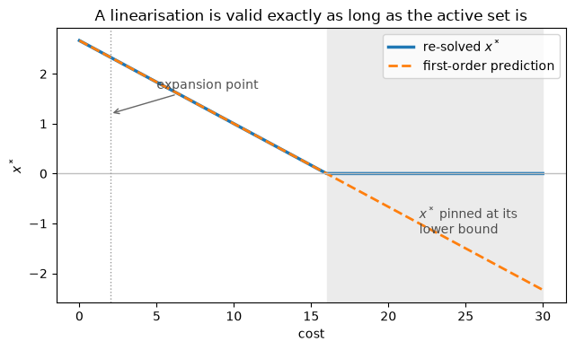
../_images/d466e450e2d10837bd6ffd1638df09f32b9b72e509b15d5ec275a7e875a4ea8e.png

Two things worth reading off that figure.

Below the switch the prediction is not approximate — it is exact. A quadratic objective with linear constraints has a solution map that is affine in the parameters while the active set holds, so the first-order term is the whole story and the two curves lie on top of each other to solver tolerance. The \(O(\|\Delta p\|^2)\) error bound is a worst case, not a fee charged on every step.

Past the switch it is not approximate either — it is wrong. At cost ≈ 16 the optimal \(x^*\) reaches its lower bound of zero and stays there; the linearisation knows nothing about that bound and marches on into negative, infeasible territory. It is not degrading gracefully, it is extrapolating a branch that no longer exists.

That is the honest limit of a first-order sensitivity, and it is why Sensitivity carries active and at_bound: they are how you check that the branch you linearised on is still the branch you are standing on.

Second order#

order=2 also assembles \(\partial^2 x^*/\partial p^2\), which lets an outer solver use an exact Hessian through the solution map instead of a quasi-Newton approximation.

On the blending model it comes back exactly zero — and that is the right answer, not a failure: a quadratic objective with linear constraints has a solution map that is affine in the parameters, so on a fixed active set \(x^*(p)\) has no curvature at all. It is worth seeing, because it is the cheapest available check that the second-order machinery is measuring something real rather than returning noise.

s2 = m.sensitivity(order=2)
print("d2x*/dp2 shape :", s2.d2x_dp2.shape, " (n_vars, n_params, n_params)")
print("for x          :\n", s2.d2x_dp2[0], " <- affine solution map, so exactly zero")

d2x*/dp2 shape : (2, 2, 2)  (n_vars, n_params, n_params)
for x          :
 [[0. 0.]
 [0. 0.]]  <- affine solution map, so exactly zero

A curved solution map to contrast: \(\min\,(x - p^2)^2\) has \(x^*(p) = p^2\), so \(\mathrm{d}x^*/\mathrm{d}p = 2p\) and \(\mathrm{d}^2x^*/\mathrm{d}p^2 = 2\) exactly. Here second order is not decoration — the first-order prediction is visibly wrong at a finite step, and the second-order one is exact.

def curved(p_value=1.5):
    mc = dm.Model("curved")
    p = mc.parameter("p", value=p_value)
    xc = mc.continuous("x", lb=-50.0, ub=50.0)
    mc.minimize((xc - p * p) ** 2)
    return mc, p, xc


mc, p, xc = curved()
sc = mc.sensitivity(order=2)

print(f"x*           = {float(sc.x_dict['x']):.6f}   (p^2 = {1.5**2:.6f})")
print(f"dx*/dp       = {float(sc.d(xc, p)):.6f}   (2p = {2 * 1.5:.6f})")
print(f"d2x*/dp2     = {float(sc.d2x_dp2[0, 0, 0]):.6f}   (exactly 2)")
print()
target_p = 2.0
print(f"at p = {target_p}:  truth = {target_p**2:.6f}")
print(f"  first order  = {float(sc.predict({p: target_p}, order=1)['x']):.6f}")
print(f"  second order = {float(sc.predict({p: target_p}, order=2)['x']):.6f}")

x*           = 2.250000   (p^2 = 2.250000)
dx*/dp       = 3.000000   (2p = 3.000000)
d2x*/dp2     = 2.000000   (exactly 2)

at p = 2.0:  truth = 4.000000
  first order  = 3.750000
  second order = 4.000000

`as_layer()` — the same map, as a JAX function#

When the model is a component of something larger — a training loop, an outer optimization — you want the solution map as a differentiable callable rather than as matrices. as_layer() hands you \(\varphi(p) \mapsto x^*\), differentiable twice, ready for jax.grad / jax.jit / jax.vmap. This is the decision-focused-learning shape [Agrawal et al., 2019, Amos and Kolter, 2017].

import jax.numpy as jnp

phi = s.as_layer()
p0 = jnp.array([float(cost.value), float(target.value)])

print("phi(p0)                :", np.asarray(phi(p0)))
print("jax.jacobian(phi)(p0)  :\n", np.asarray(jax.jacobian(phi)(p0)))
print("matches s.dx_dp        :", np.allclose(np.asarray(jax.jacobian(phi)(p0)), s.dx_dp, atol=1e-6))

phi(p0)                : [2.33333333 1.66666666]

jax.jacobian(phi)(p0)  :
 [[-0.16666667  0.66666667]
 [ 0.16666667  0.33333333]]

matches s.dx_dp        : True

6. The other direction: a derivative inside a model#

Everything so far differentiates a model from outside. The complementary tool puts an implicitly defined quantity into one: Model.implicit defines \(v\) by \(g(u, v) = 0\) and supplies the solver with \(\mathrm{d}v/\mathrm{d}u = -(\partial g/\partial v)^{-1}(\partial g/\partial u)\) — the same implicit function theorem, used at model-build time rather than at post-solve time. Newton runs forward; nothing differentiates through its iterations.

dm.argmin does the same for a whole inner NLP, making a follower’s minimizer a block of an outer model. Both ride on the CustomCall contract: the outer model is solved on the local NLP path only, with no global certificate and no integer variables. The Implicit function node notebook covers the first in full; dm.argmin’s docstring covers the second, including why hand-writing a nonconvex follower’s KKT conditions instead is a relaxation rather than a reformulation.

import jax.numpy as jnp

mi = dm.Model("implicit_demo")
u = mi.continuous("u", lb=0.1, ub=100.0)
v = mi.implicit(lambda U, V: jnp.array([V[0] ** 2 - U[0]]), [u], n_unknowns=1,
                x0=jnp.array([1.0]))
mi.minimize((v[0] - 3.0) ** 2)     # v = sqrt(u); optimum at u = 9

ri = mi.solve()
print(f"status = {ri.status}   u* = {float(ri.x['u']):.6f}   (expected 9)")

No valid dual bound was produced for model 'implicit_demo': the relaxation layer could not bound this objective (status=feasible). The result cannot be certified globally optimal. A nonlinear term with no envelope is the usual cause; an epigraph reformulation (minimize z subject to f(x) <= z) often gives the relaxation something to bound.

status = feasible   u* = 9.000000   (expected 9)

Summary#

Question	Call
Slope of an expression, symbolically	`diff(expr, x)`, `grad(expr, [x, y])`
Partials \(\partial e/\partial x\), \(\partial e/\partial p\)	`compile_expression(expr, m)` + `jax.grad`
How the optimum value moves	`m.solve(sensitivity=True)` → `result.gradient(p)`
How the solution moves, and everything else	`m.sensitivity()`
Raw sIPOPT arrays	`pounce_sensitivity(m, [p])`
The solution map as a JAX function	`s.as_layer()`, `dm.argmin_layer(m, [p])`
An implicit function inside a model	`m.implicit(residual, [u], n_unknowns=k)`
An inner NLP inside a model	`dm.argmin(inner, bind={p: outer_expr})`

Contract for everything in the bottom half of that table: continuous variables only, scalar parameters only, and the derivatives describe the KKT point the solver returned — for a nonconvex model, a local one, on the active-set branch recorded in s.active / s.at_bound.

Full citation details for the works above are on the references page.