One model, four jobs: simulate, fit, design, optimize

A model is the durable thing. Simulation, regression, design of experiments and optimization are not four models — they are four questions put to the same one. What changes between them is only

• which quantities are free, and

• what is being optimized.

This notebook makes that literal. The reactor is written down once as a discopt Model, and then the same model is simulated, regressed, designed on, and optimized. Between stages it does not stay in memory: it is serialized to a file and loaded back, the way a calibrated model travels between the study that produced it and the work that uses it [Wilkinson et al., 2016].

job	free	fixed	objective
simulate	the state \(C_A, C_B, C_C\)	\(k_1, k_2\), \(F\)	none — a square solve
regress	\(k_1, k_2\)	\(F\) at each measured condition	min weighted SSE
design (MBDoE)	\(F\)	\(k_1, k_2\) at \(\hat\theta\)	max \(\det \mathrm{FIM}\)
optimize	\(F\)	\(k_1, k_2\) at \(\hat\theta\)	max \(C_B\)

The statistical background is Bard [1974] and Biegler [2010]; for MBDoE see Franceschini and Macchietto [2008] and Atkinson et al. [2007], with the original non-linear design argument in Box and Lucas [1959].

Note

The design section needs the optional plugin: pip install discopt-doe.

The data comes from a file, not from this notebook. cstr_lab.py, next to this notebook, is the “laboratory”: it owns the true rate constants and the measurement noise, and writes CSV assay files. Nothing here imports it, so the notebook cannot read the answer it is meant to estimate. At the very end we ask it to open the envelope.

import json
import subprocess
import sys
from pathlib import Path

import matplotlib.pyplot as plt
import numpy as np
from IPython.display import Markdown

import discopt
import discopt.modeling as dm
from discopt import doe
from discopt.estimate import Experiment, ExperimentModel, estimate_parameters

# Executed from this notebook's directory (jupyter-book) or from the repo root.
HERE = Path.cwd() if (Path.cwd() / "cstr_lab.py").exists() else Path("docs/notebooks")
LAB = HERE / "cstr_lab.py"
DATA = HERE / "data"
CALIBRATED_V1 = HERE / "cstr_calibrated_v1.dopt"
CALIBRATED_V2 = HERE / "cstr_calibrated_v2.dopt"
assert LAB.exists(), f"cannot find the lab script from {Path.cwd()}"

plt.rcParams.update({"figure.dpi": 110, "font.size": 10, "figure.autolayout": True})

1. Write the model down once

A single isothermal CSTR of volume \(V\), fed pure A at concentration \(C_{A0}\) and volumetric flow rate \(F\), with the first-order series reaction

\[\mathrm{A} \xrightarrow{k_1} \mathrm{B} \xrightarrow{k_2} \mathrm{C}.\]

With residence time \(\tau = V/F\), the steady-state balances \(F(C_{A0}-C_A) = V k_1 C_A\) and \(F(0-C_B) = V(k_2 C_B - k_1 C_A)\) solve in closed form [Fogler, 2016]:

\[C_A = \frac{C_{A0}}{1+k_1\tau}, \qquad C_B = \frac{k_1 \tau\, C_{A0}}{(1+k_1\tau)(1+k_2\tau)}, \qquad C_C = C_{A0} - C_A - C_B .\]

In the model, everything is a variable: the state \(C_A, C_B, C_C\), the operating condition \(F\), and the rate constants \(k_1, k_2\). The three equations above go in as named equality rows. Nothing in the model says which of these is known — that is the job’s choice, made later by pinning bounds, and it is the only thing that changes from section to section.

The reactor’s own specification — volume, feed concentration, and the assay’s repeatability — are Parameters: values that are fixed during a solve but can be re-valued between solves. Two more parameters, fim and n_obs, carry what we learn about \(k_1, k_2\) from the data; they appear in no equation, and they are parameters because that is the slot discopt’s file format keeps for a model’s own numbers (§5).

n_runs is the only structural knob: one instance of the reactor, or \(n\) of them sharing one pair of rate constants — which is exactly what a campaign of \(n\) runs is.

def build_reactor(n_runs=1, name="cstr"):
    """The reactor, as a model. `n_runs` copies share one pair of rate constants."""
    m = dm.Model(name)

    V = m.parameter("V", 1.0)  # reactor volume, L
    CA0 = m.parameter("CA0", 2.0)  # feed concentration of A, mol/L
    m.parameter("sigma", 0.03)  # assay repeatability, mol/L
    m.parameter("fim", np.zeros((2, 2)))  # Fisher information about (k1, k2)
    m.parameter("n_obs", 0.0)  # observations behind that information

    shape = () if n_runs == 1 else (n_runs,)
    k1 = m.continuous("k1", lb=1e-3, ub=20.0)  # 1/min
    k2 = m.continuous("k2", lb=1e-3, ub=20.0)  # 1/min
    F = m.continuous("F", shape=shape, lb=0.05, ub=5.0)  # L/min
    CA = m.continuous("CA", shape=shape, lb=0.0, ub=10.0)  # mol/L
    CB = m.continuous("CB", shape=shape, lb=0.0, ub=10.0)
    CC = m.continuous("CC", shape=shape, lb=0.0, ub=10.0)

    tau = V / F
    m.subject_to(CA == CA0 / (1.0 + k1 * tau), name="CA_def")
    m.subject_to(CB == k1 * tau * CA0 / ((1.0 + k1 * tau) * (1.0 + k2 * tau)), name="CB_def")
    m.subject_to(CC == CA0 - CA - CB, name="CC_def")
    return m


def parts(m):
    """Variables, parameters and rows of `m`, by name -- also after a reload."""
    return (
        {v.name: v for v in m._variables},
        {p.name: p for p in m._parameters},
        {c.name: c for c in m._constraints},
    )


reactor = build_reactor()
var, par, row = parts(reactor)
print(reactor.summary())
print("\nrows:", list(row))

Model: cstr
  Variables: 6 (6 continuous, 0 integer/binary)
  Constraints: 3
  Objective: <none set>
  Parameters: 5

rows: ['CA_def', 'CB_def', 'CC_def']

One more thing the model has to hand back

Design of experiments needs the responses as explicit functions of the parameters: the Fisher information is built from \(\partial y/\partial\theta\) by autodiff through the response expression, so a bare CA variable — whose derivative with respect to \(k_1\) is zero — would silently produce a singular information matrix and a meaningless covariance.

The closed forms are already in the model, inside the definition rows. discopt normalizes a row y == expr to the body y - expr, so the response expression comes back as y - body. That is one line, it works on a model that was just built and on one that was just read from disk, and it means the expression is never written a second time.

It prints as y - (y - expr), because the DAG is stored as built and nothing simplifies it. That costs two extra nodes and nothing else: the two y terms cancel in the derivative, so \(\partial y/\partial\theta\) is exactly the derivative of the closed form.

def responses(m):
    """The closed-form response expressions, recovered from the definition rows."""
    v, _, rows = parts(m)
    return {y: v[y] - rows[f"{y}_def"].body for y in ("CA", "CB", "CC")}


print("row body:", row["CA_def"].body)
print("response:", responses(reactor)["CA"])

row body: (CA - (param(CA0) / (1 + (k1 * (param(V) / F)))))
response: (CA - (CA - (param(CA0) / (1 + (k1 * (param(V) / F))))))

2. Simulate — no degrees of freedom left

Fix the rate constants and the flow rate and there is nothing left to choose: the three rows determine the state. That is a square problem, so the objective is a constant — we are asking for feasibility, not for a best point.

Model.fixed sets lb == ub for the duration of the block and restores the bounds on exit. Scoping matters: bounds are re-read at every solve, so a fix left behind by accident would silently redefine the next problem and still report optimal.

reactor.minimize(0.0)  # a square solve: satisfy the balances, optimize nothing


def simulate(m, k1, k2, flows):
    """Outlet concentrations at each flow rate, by solving the model."""
    v, _, _ = parts(m)
    out = []
    for F in np.atleast_1d(flows):
        with m.fixed({v["k1"]: k1, v["k2"]: k2, v["F"]: float(F)}):
            r = m.solve(time_limit=30)
        if r.status != "optimal":
            raise RuntimeError(f"simulation at F={F} returned {r.status}")
        out.append([float(r.value(v[y])) for y in ("CA", "CB", "CC")])
    return np.array(out)


GUESS = {"k1": 0.5, "k2": 1.0}  # what we believe before seeing any data
CA_s, CB_s, CC_s = simulate(reactor, GUESS["k1"], GUESS["k2"], 1.0)[0]
print(f"at F = 1.0 L/min and the prior guess {GUESS}:")
print(f"  C_A = {CA_s:.4f}   C_B = {CB_s:.4f}   C_C = {CC_s:.4f}  mol/L")
print(f"  mass balance: C_A + C_B + C_C = {CA_s + CB_s + CC_s:.6f} (feed is 2.0)")

at F = 1.0 L/min and the prior guess {'k1': 0.5, 'k2': 1.0}:
  C_A = 1.3333   C_B = 0.3333   C_C = 0.3333  mol/L
  mass balance: C_A + C_B + C_C = 2.000000 (feed is 2.0)

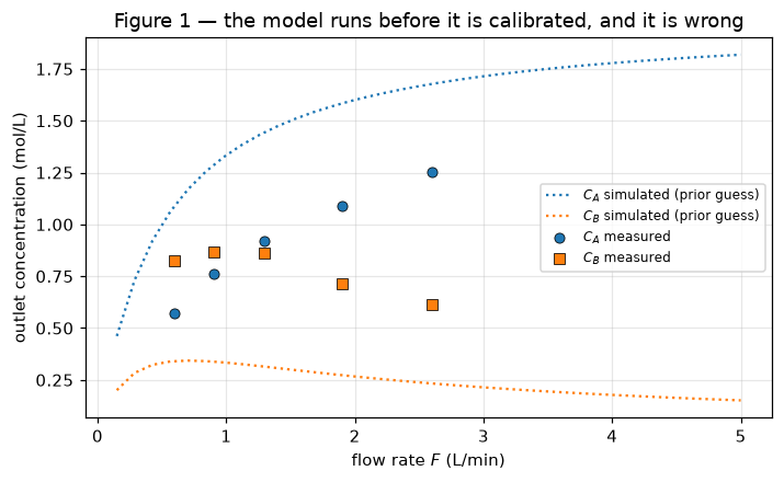
3. The data

cstr_lab.py wrote the first campaign — five flow rates over a fairly narrow, conveniently fast range. Its header records the rig; the true rate constants stay inside the script.

def read_assay(path):
    """Rows of a cstr_lab.py assay file. Its '#' lines carry the rig's spec."""
    text = Path(path).read_text()
    body = [ln for ln in text.splitlines() if not ln.startswith("#")]
    return np.atleast_1d(np.genfromtxt(body, delimiter=",", names=True))


print((DATA / "cstr_campaign1.csv").read_text())
campaign = read_assay(DATA / "cstr_campaign1.csv")

# Steady-state CSTR assay, written by cstr_lab.py
# rig: V=1.0 L, CA0=2.0 mol/L
# F: L/min; CA, CB, sigma: mol/L
F,CA,CB,sigma
0.600000,0.571465,0.827393,0.030000
0.900000,0.758962,0.867189,0.030000
1.300000,0.920347,0.859534,0.030000
1.900000,1.090929,0.714134,0.030000
2.600000,1.254653,0.615532,0.030000

F_dense = np.linspace(0.15, 5.0, 36)
prior_profile = simulate(reactor, GUESS["k1"], GUESS["k2"], F_dense)

fig, ax = plt.subplots(figsize=(6.6, 4.1))
ax.plot(F_dense, prior_profile[:, 0], color="C0", ls=":", label="$C_A$ simulated (prior guess)")
ax.plot(F_dense, prior_profile[:, 1], color="C1", ls=":", label="$C_B$ simulated (prior guess)")
ax.plot(campaign["F"], campaign["CA"], "o", color="C0", mec="k", mew=0.5, label="$C_A$ measured")
ax.plot(campaign["F"], campaign["CB"], "s", color="C1", mec="k", mew=0.5, label="$C_B$ measured")
ax.set_xlabel("flow rate $F$ (L/min)")
ax.set_ylabel("outlet concentration (mol/L)")
ax.set_title("Figure 1 — the model runs before it is calibrated, and it is wrong")
ax.legend(fontsize=8)
ax.grid(alpha=0.3)
plt.show()

4. Regress — free the rate constants, pin the flow rates

Same model, five copies of it (n_runs=5) sharing one pair of rate constants. The flow rates are pinned at what was actually run — lb == ub is how a fixed variable is expressed — and \(k_1, k_2\) are the only things left free. The objective becomes the weighted sum of squared residuals.

discopt.estimate wants an Experiment whose create_model() returns an ExperimentModel labelling what is unknown, what was controlled and what was measured. Each run contributes two responses, \(C_A\) and \(C_B\), both taken straight off the model with responses().

class Campaign(Experiment):
    """n runs of the reactor at known flow rates -- the regression view."""

    def __init__(self, flows, sigma):
        self.flows = np.asarray(flows, dtype=float)
        self.sigma = np.asarray(sigma, dtype=float)

    def create_model(self, **guess):
        m = build_reactor(len(self.flows), name="cstr_campaign")
        v, _, _ = parts(m)

        v["F"].lb = self.flows.copy()  # pin the conditions that were run
        v["F"].ub = self.flows.copy()
        start = {v[name]: float(val) for name, val in guess.items() if name in v}
        if start:
            m.set_initial_point(start)

        y = responses(m)
        resp, err = {}, {}
        for i in range(len(self.flows)):
            for name in ("CA", "CB"):
                resp[f"{name}_{i}"] = y[name][i]
                err[f"{name}_{i}"] = float(self.sigma[i])
        return ExperimentModel(
            model=m,
            unknown_parameters={"k1": v["k1"], "k2": v["k2"]},
            design_inputs={},
            responses=resp,
            measurement_error=err,
        )


def observations(rows):
    """Assay rows -> the {response_name: value} dict estimate_parameters wants."""
    return {
        f"{name}_{i}": float(rows[name][i])
        for i in range(len(rows["F"]))
        for name in ("CA", "CB")
    }


fit_1 = estimate_parameters(
    Campaign(campaign["F"], campaign["sigma"]),
    observations(campaign),
    initial_guess=GUESS,
)
print(fit_1.summary())

No valid dual bound was produced for model 'cstr_campaign': the relaxation layer could not bound this objective (status=feasible). The result cannot be certified globally optimal. A nonlinear term with no envelope is the usual cause; an epigraph reformulation (minimize z subject to f(x) <= z) often gives the relaxation something to bound.

Parameter Estimation Results
==================================================
            k1 =      1.52528  ± 0.04033  [1.432, 1.618]
            k2 =     0.417587  ± 0.0284  [0.3521, 0.4831]
     Objective = 4.04436
         N obs = 10
       FIM det = 1.016e+06
      FIM cond = 3.746

Note

discopt reports that it could not certify this fit globally. That is expected and not a failure: nonlinear least squares is run as a local NLP (skip_convex_check=True), because spatial branch-and-bound over a sum-of-squares surface is rarely what a fit wants. The optimization in §7, where the certificate does matter, is a global solve.

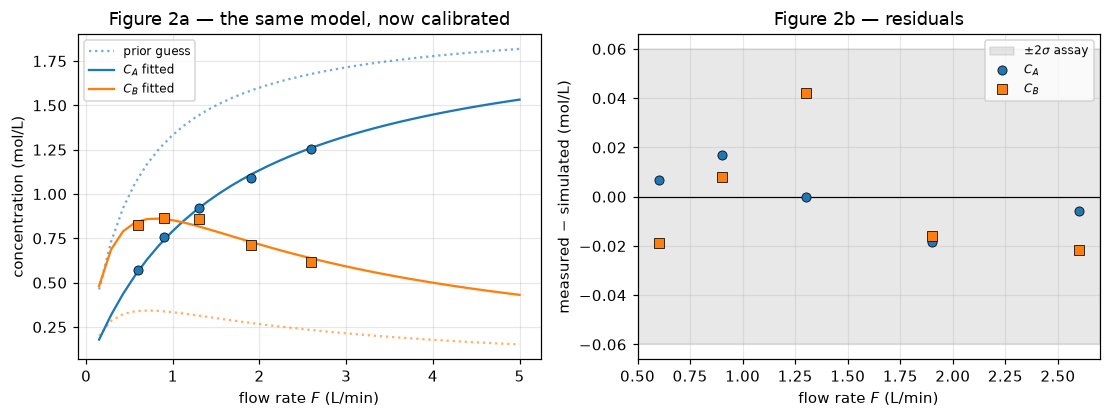
Parameters and uncertainties after campaign 1

EstimationResult carries the covariance — the inverse Fisher information at the solution — so standard errors, 95% confidence intervals and the parameter correlation all come straight off the fit.

def parameter_table(fit, title=""):
    """Render an estimate +/- uncertainty table as Markdown."""
    se, ci = fit.standard_errors, fit.confidence_intervals
    rows = [
        "| parameter | estimate | std. error | 95% CI | rel. error |",
        "|---|---:|---:|:---:|---:|",
    ]
    for name in fit.parameter_names:
        val, s = fit.parameters[name], se[name]
        lo, hi = ci[name]
        rows.append(
            f"| ${name[0]}_{name[1]}$ | {val:.4f} | {s:.4f} | "
            f"[{lo:.4f}, {hi:.4f}] | {100 * s / abs(val):.2f}% |"
        )
    return Markdown(
        f"**{title}**\n\n" + "\n".join(rows) + f"\n\n*Weighted SSE = {fit.objective:.4f} on "
        f"{fit.n_observations} observations; "
        f"corr($k_1$,$k_2$) = {fit.correlation_matrix[0, 1]:+.3f}.*"
    )


parameter_table(fit_1, "Table 1 — campaign 1 (5 flow rates, 10 observations)")

Table 1 — campaign 1 (5 flow rates, 10 observations)

| parameter | estimate | std. error | 95% CI | rel. error | |—|—:|—:|:—:|—:| | $k_1$ | 1.5253 | 0.0403 | [1.4323, 1.6183] | 2.64% | | $k_2$ | 0.4176 | 0.0284 | [0.3521, 0.4831] | 6.80% |

Weighted SSE = 4.0444 on 10 observations; corr($k_1$,$k_2$) = +0.500.

fitted_profile = simulate(reactor, fit_1.parameters["k1"], fit_1.parameters["k2"], F_dense)
at_runs = simulate(reactor, fit_1.parameters["k1"], fit_1.parameters["k2"], campaign["F"])

fig, axes = plt.subplots(1, 2, figsize=(10.2, 3.9))

ax = axes[0]
ax.plot(F_dense, prior_profile[:, 0], color="C0", ls=":", alpha=0.6, label="prior guess")
ax.plot(F_dense, prior_profile[:, 1], color="C1", ls=":", alpha=0.6)
ax.plot(F_dense, fitted_profile[:, 0], color="C0", label="$C_A$ fitted")
ax.plot(F_dense, fitted_profile[:, 1], color="C1", label="$C_B$ fitted")
ax.plot(campaign["F"], campaign["CA"], "o", color="C0", mec="k", mew=0.5)
ax.plot(campaign["F"], campaign["CB"], "s", color="C1", mec="k", mew=0.5)
ax.set_xlabel("flow rate $F$ (L/min)")
ax.set_ylabel("concentration (mol/L)")
ax.set_title("Figure 2a — the same model, now calibrated")
ax.legend(fontsize=8)
ax.grid(alpha=0.3)

ax = axes[1]
sigma = float(campaign["sigma"][0])
ax.axhline(0, color="k", lw=0.8)
ax.axhspan(-2 * sigma, 2 * sigma, color="grey", alpha=0.18, label=r"$\pm 2\sigma$ assay")
ax.plot(campaign["F"], campaign["CA"] - at_runs[:, 0], "o", color="C0", mec="k", mew=0.5, label="$C_A$")
ax.plot(campaign["F"], campaign["CB"] - at_runs[:, 1], "s", color="C1", mec="k", mew=0.5, label="$C_B$")
ax.set_xlabel("flow rate $F$ (L/min)")
ax.set_ylabel("measured $-$ simulated (mol/L)")
ax.set_title("Figure 2b — residuals")
ax.legend(fontsize=8)
ax.grid(alpha=0.3)
plt.show()

5. Serialize the calibrated model

The campaign model was scaffolding — five reactors tied to one pair of rate constants, useful for one afternoon. What we want to keep is the reactor, calibrated: one instance, carrying what the data taught us.

Three things travel in the file:

• the model itself — variables, bounds, the named definition rows, the rig’s parameters;

• \(\hat\theta\), as the model’s initial point, which is exactly what a start value is: the current best estimate of \(k_1\) and \(k_2\);

• the Fisher information and the observation count, in the fim and n_obs parameters — enough to reconstruct the covariance, the confidence intervals, and the prior for the next design.

Model.save writes a single JSON document [Fourer et al., 2003] — greppable, diffable, with no pickle and no numpy version baked in — plus a provenance block recording what wrote it and when.

def save_calibrated(path, fit):
    """Write the reactor with this fit's estimates and information attached."""
    m = build_reactor(1)
    v, p, _ = parts(m)
    m.set_initial_point({v["k1"]: fit.parameters["k1"], v["k2"]: fit.parameters["k2"]})
    p["fim"].value = fit.fim
    p["n_obs"].value = float(fit.n_observations)
    m.save(path, indent=2)
    return path


save_calibrated(CALIBRATED_V1, fit_1)
print(f"{CALIBRATED_V1.name}: {CALIBRATED_V1.stat().st_size} bytes")
print("\n".join(CALIBRATED_V1.read_text().splitlines()[:12]))

cstr_calibrated_v1.dopt: 4741 bytes
{
  "schema": "discopt.model/1.3",
  "discopt": "0.9.0",
  "name": "cstr",
  "variables": [
    {
      "name": "k1",
      "type": "continuous",
      "shape": [],
      "lb": 0.001,
      "ub": 20.0,
      "bound_stack": []

6. Load it back and design the next experiment

A fresh read from disk. Nothing below uses fit_1 or reactor — everything the next stage needs is in the file.

def estimate_from(m):
    """The parameter estimates a calibrated model carries, from its start point."""
    v, _, _ = parts(m)
    return {name: m.initial_point[v[name]][0] for name in ("k1", "k2")}


def information_from(m):
    """(Fisher information, observation count) carried by a calibrated model."""
    _, p, _ = parts(m)
    return np.asarray(p["fim"].value, dtype=float), int(p["n_obs"].value)


restored = discopt.load(CALIBRATED_V1)
theta_hat = estimate_from(restored)
prior_fim, n_obs = information_from(restored)

print(restored.summary())
print("\nwritten by:", restored.provenance["software"])
print("estimates carried:", {k: round(v, 6) for k, v in theta_hat.items()})
print(f"prior information ({n_obs} observations):\n{prior_fim}")
print(f"\nimplied std. errors: {np.sqrt(np.diag(np.linalg.inv(prior_fim))).round(5)}")

Model: cstr
  Variables: 6 (6 continuous, 0 integer/binary)
  Constraints: 3
  Objective: <none set>
  Parameters: 5

written by: {'name': 'discopt', 'version': '0.9.0', 'rust_core': '0.2.0', 'repository': 'https://github.com/jkitchin/discopt', 'license': 'EPL-2.0'}
estimates carried: {'k1': 1.525276, 'k2': 0.417587}
prior information (10 observations):
[[ 819.36664978 -581.25980175]
 [-581.25980175 1652.40226739]]

implied std. errors: [0.04033 0.0284 ]

Which flow rate should we run next? MBDoE answers by asking which condition adds the most Fisher information about the parameters [Franceschini and Macchietto, 2008]:

\[\mathrm{FIM} = J^\top \Sigma^{-1} J, \qquad J_{ij} = \frac{\partial y_i}{\partial \theta_j},\]

evaluated at the current best estimate \(\hat\theta\) — sensitivities that discopt-doe gets by autodiff, not finite differences. We maximize \(\det(\mathrm{FIM}_{\text{prior}} + \mathrm{FIM}_{\text{new}})\) (the D-optimal criterion), passing the information from the file as the prior, so the design is genuinely sequential.

This is the third job, and the free/fixed partition has flipped again: \(F\) is now the unknown and \(k_1, k_2\) are held at \(\hat\theta\). The Experiment below builds its model by loading the file — the physics is not written again.

class SavedReactor(Experiment):
    """A calibrated reactor read from disk, with F as the DESIGN variable."""

    def __init__(self, path):
        self.path = str(path)

    def create_model(self, **kwargs):
        m = discopt.load(self.path)
        v, p, _ = parts(m)
        y = responses(m)
        sigma = float(p["sigma"].value)
        return ExperimentModel(
            model=m,
            unknown_parameters={"k1": v["k1"], "k2": v["k2"]},
            design_inputs={"F": v["F"]},
            responses={"CA": y["CA"], "CB": y["CB"]},
            measurement_error={"CA": sigma, "CB": sigma},
        )


design_view = SavedReactor(CALIBRATED_V1)
F_BOUNDS = (0.05, 5.0)

best = doe.optimal_experiment(
    design_view,
    param_values=theta_hat,
    design_bounds={"F": F_BOUNDS},
    criterion="determinant",
    prior_fim=prior_fim,
    seed=1,
)
F_next = float(best.design["F"])
print(f"D-optimal next flow rate: F = {F_next:.4f} L/min  (tau = {1.0 / F_next:.3f} min)")
print(f"log det(FIM) there      : {best.criterion_value:.4f}")

D-optimal next flow rate: F = 0.3116 L/min  (tau = 3.210 min)
log det(FIM) there      : 14.4537

Why that flow rate?

Scanning the criterion over the whole feasible range shows the design landscape rather than just its argmax — worth plotting, because a flat optimum means the exact recommendation hardly matters, while a sharp one means it does.

F_grid = np.linspace(F_BOUNDS[0], F_BOUNDS[1], 60)
fims = [doe.compute_fim(design_view, theta_hat, {"F": float(F)}) for F in F_grid]
logdet = np.array([np.log(np.linalg.det(prior_fim + f.fim)) for f in fims])

# What a sixth run is worth, by where you put it: det(FIM) after, over det(FIM) now.
ld_prior = np.log(np.linalg.det(prior_fim))


def worth(F):
    fim = doe.compute_fim(design_view, theta_hat, {"F": float(F)}).fim
    return np.exp(np.log(np.linalg.det(prior_fim + fim)) - ld_prior)


covered = (F_grid >= campaign["F"].min()) & (F_grid <= campaign["F"].max())
candidates = [
    ("the D-optimal design", F_next),
    ("best F campaign 1 covers", float(F_grid[covered][np.argmax(logdet[covered])])),
    ("repeat the middle run", float(campaign["F"][len(campaign["F"]) // 2])),
    ("repeat the fastest run", float(campaign["F"].max())),
    ("the slowest F allowed", float(F_grid[0])),
]
print(f"det(FIM) now: {np.exp(ld_prior):.4g}. A sixth run multiplies it by\n")
for label, F in candidates:
    print(f"  {label:<26s} F = {F:5.3f} L/min   {worth(F):.2f}x")

fig, axes = plt.subplots(1, 2, figsize=(10.2, 3.9))

ax = axes[0]
ax.plot(F_grid, logdet, color="C4")
ax.axvline(F_next, color="C3", ls="--", label=f"D-optimal $F$ = {F_next:.3f}")
for F in campaign["F"]:
    ax.axvline(F, color="grey", alpha=0.45, lw=0.9)
ax.plot([], [], color="grey", alpha=0.45, lw=0.9, label="campaign 1 points")
ax.set_xlabel("candidate flow rate $F$ (L/min)")
ax.set_ylabel(r"$\log\det(\mathrm{FIM}_{\rm prior} + \mathrm{FIM}(F))$")
ax.set_title("Figure 3a — D-optimal design criterion")
ax.legend(fontsize=8)
ax.grid(alpha=0.3)

ax = axes[1]
J = np.array([f.jacobian for f in fims])
for r, resp in enumerate(fims[0].response_names):
    for p_i, par_name in enumerate(["k_1", "k_2"]):
        ax.plot(F_grid, np.abs(J[:, r, p_i]),
                label=rf"$|\partial {resp[0]}_{resp[1]}/\partial {par_name}|$")
ax.axvline(F_next, color="C3", ls="--")
ax.set_xlabel("flow rate $F$ (L/min)")
ax.set_ylabel("sensitivity magnitude")
ax.set_title("Figure 3b — why: parameter sensitivities")
ax.legend(fontsize=8)
ax.grid(alpha=0.3)
plt.show()

det(FIM) now: 1.016e+06. A sixth run multiplies it by

  the D-optimal design       F = 0.312 L/min   1.86x
  best F campaign 1 covers   F = 0.637 L/min   1.66x

  repeat the middle run      F = 1.300 L/min   1.38x
  repeat the fastest run     F = 2.600 L/min   1.27x
  the slowest F allowed      F = 0.050 L/min   1.18x

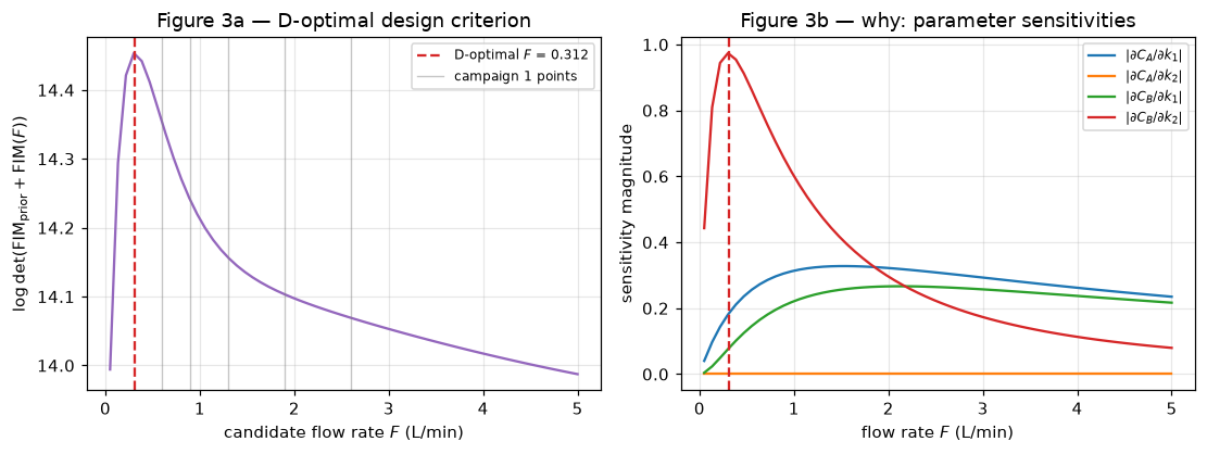
The recommendation is a low flow rate — a long residence time — but not the lowest on offer: the optimum is interior, and the criterion falls away on both sides of it.

Each side fails for its own reason, and the right panel shows both. Run fast and the second reaction barely gets started, so \(C_B\) hardly moves with \(k_2\); that is the blind spot campaign 1 was sitting in, and it is why \(k_2\) came out of it with roughly two and a half times \(k_1\)’s relative error (Table 1). Run slow enough and the reactor goes essentially to completion — at the slowest allowed setting the model predicts an outlet of \(C_A \approx 0.06\), \(C_B \approx 0.21\) out of a 2.0 mol/L feed — and an outlet that is nearly all C is insensitive to how fast it got there. Between the two, \(|\partial C_B/\partial k_2|\) peaks, and that is where the design landed.

The table above the figure prices the alternatives. The gain is real but not dramatic: no single sixth run transforms this campaign, and simply repeating a condition already covered is worth a good deal of it. What the design buys is the direction of the improvement — it goes after \(k_2\), the parameter campaign 1 left loose, rather than piling more evidence onto \(k_1\), which was already the well-determined one. Table 3 below is where that shows up.

Send it to the lab

The design goes out as a request for one run at one flow rate, and comes back as another assay file.

run_6 = DATA / "cstr_run6.csv"
completed = subprocess.run(
    [sys.executable, str(LAB), "--flows", f"{F_next:.4f}", "--seed", "11", "--out", str(run_6)],
    check=True,
    capture_output=True,
    text=True,
)
print(completed.stdout, end="")

new_run = read_assay(run_6)
refined = {k: np.concatenate([campaign[k], new_run[k]]) for k in ("F", "CA", "CB", "sigma")}

wrote 1 run(s) to /Users/jkitchin/projects/discopt/docs/notebooks/data/cstr_run6.csv
  F =  0.312 L/min   CA =  0.3450   CB =  0.7659  mol/L

Refit with all six runs

Back to the regression, unchanged except that the campaign now has six members. The previous estimates seed the solve.

fit_2 = estimate_parameters(
    Campaign(refined["F"], refined["sigma"]),
    observations(refined),
    initial_guess=theta_hat,
)
parameter_table(fit_2, "Table 2 — after the designed run (6 flow rates, 12 observations)")

No valid dual bound was produced for model 'cstr_campaign': the relaxation layer could not bound this objective (status=feasible). The result cannot be certified globally optimal. A nonlinear term with no envelope is the usual cause; an epigraph reformulation (minimize z subject to f(x) <= z) often gives the relaxation something to bound.

Table 2 — after the designed run (6 flow rates, 12 observations)

| parameter | estimate | std. error | 95% CI | rel. error | |—|—:|—:|:—:|—:| | $k_1$ | 1.5091 | 0.0372 | [1.4262, 1.5919] | 2.46% | | $k_2$ | 0.3914 | 0.0203 | [0.3462, 0.4366] | 5.19% |

Weighted SSE = 6.0254 on 12 observations; corr($k_1$,$k_2$) = +0.437.

rows = [
    "| parameter | SE before | SE after | change | 95% CI width before | after |",
    "|---|---:|---:|---:|---:|---:|",
]
for name in fit_1.parameter_names:
    s1, s2 = fit_1.standard_errors[name], fit_2.standard_errors[name]
    w1 = np.diff(fit_1.confidence_intervals[name])[0]
    w2 = np.diff(fit_2.confidence_intervals[name])[0]
    rows.append(
        f"| ${name[0]}_{name[1]}$ | {s1:.5f} | {s2:.5f} | "
        f"{100 * (s2 - s1) / s1:+.1f}% | {w1:.4f} | {w2:.4f} |"
    )
d1, d2 = np.linalg.det(fit_1.fim), np.linalg.det(fit_2.fim)
Markdown(
    "**Table 3 — what the single designed experiment bought**\n\n"
    + "\n".join(rows)
    + f"\n\n*det(FIM): {d1:.4g} → {d2:.4g} ({d2 / d1:.2f}×). "
    "One extra run, chosen by the model.*"
)

Table 3 — what the single designed experiment bought

| parameter | SE before | SE after | change | 95% CI width before | after | |—|—:|—:|—:|—:|—:| | $k_1$ | 0.04033 | 0.03719 | -7.8% | 0.1860 | 0.1657 | | $k_2$ | 0.02840 | 0.02030 | -28.5% | 0.1310 | 0.0905 |

det(FIM): 1.016e+06 → 2.169e+06 (2.13×). One extra run, chosen by the model.

Serialize the refined model

Same writer, new numbers: a second file, so the two calibrations can be compared side by side rather than one overwriting the other.

save_calibrated(CALIBRATED_V2, fit_2)

before, after = discopt.load(CALIBRATED_V1), discopt.load(CALIBRATED_V2)
t1, t2 = estimate_from(before), estimate_from(after)
cov1 = np.linalg.inv(information_from(before)[0])
cov2 = np.linalg.inv(information_from(after)[0])

print(f"{'':>4} {'v1 (5 runs)':>22} {'v2 (6 runs)':>22}")
for name in ("k1", "k2"):
    i = ("k1", "k2").index(name)
    print(f"{name:>4} {t1[name]:12.5f} +/- {np.sqrt(cov1[i, i]):.5f} "
          f"{t2[name]:12.5f} +/- {np.sqrt(cov2[i, i]):.5f}")
print(f"\nfiles on disk: {CALIBRATED_V1.name}, {CALIBRATED_V2.name}")

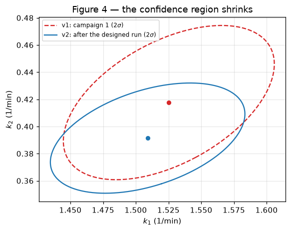
                v1 (5 runs)            v2 (6 runs)
  k1      1.52528 +/- 0.04033      1.50907 +/- 0.03719
  k2      0.41759 +/- 0.02840      0.39141 +/- 0.02030

files on disk: cstr_calibrated_v1.dopt, cstr_calibrated_v2.dopt

def confidence_ellipse(cov, center, n_std=2.0, n_points=256):
    """Points on the ``n_std``-sigma ellipse of a 2x2 covariance matrix."""
    vals, vecs = np.linalg.eigh(np.asarray(cov, dtype=float))
    t = np.linspace(0.0, 2.0 * np.pi, n_points)
    pts = vecs @ (n_std * np.sqrt(np.maximum(vals, 0.0))[:, None] * np.stack([np.cos(t), np.sin(t)]))
    return pts[0] + center[0], pts[1] + center[1]


c1, c2 = (t1["k1"], t1["k2"]), (t2["k1"], t2["k2"])
fig, ax = plt.subplots(figsize=(5.4, 4.3))
ax.plot(*confidence_ellipse(cov1, c1), color="C3", ls="--", label=r"v1: campaign 1 ($2\sigma$)")
ax.plot(*c1, "o", color="C3", ms=5)
ax.plot(*confidence_ellipse(cov2, c2), color="C0", label=r"v2: after the designed run ($2\sigma$)")
ax.plot(*c2, "o", color="C0", ms=5)
ax.set_xlabel("$k_1$ (1/min)")
ax.set_ylabel("$k_2$ (1/min)")
ax.set_title("Figure 4 — the confidence region shrinks")
ax.legend(fontsize=8)
ax.grid(alpha=0.3)
plt.show()

7. Load the refined model and optimize the flow rate

The last job. We want the flow rate that maximizes the outlet concentration of the intermediate B, with the rate constants now known — fixed at their estimates — and \(F\) free. That is the mirror image of the regression, where the \(k\)’s were free and \(F\) was pinned at whatever we happened to run.

Nothing is rebuilt: the model comes off disk, gets an objective, and is solved. Unlike the fit, this one is a global solve — spatial branch and bound over the model’s own rows — so the answer arrives with a certificate.

final = discopt.load(CALIBRATED_V2)
fv, _, _ = parts(final)
theta_final = estimate_from(final)

final.maximize(fv["CB"])  # the only new thing in the model

with final.fixed({fv["k1"]: theta_final["k1"], fv["k2"]: theta_final["k2"]}):
    opt = final.solve(time_limit=120)

F_opt = float(opt.value(fv["F"]))
CB_opt = float(opt.objective)

print(f"status        : {opt.status}   (gap certified: {opt.gap_certified})")
print(f"nodes         : {opt.node_count}")
print(f"optimal F*    : {F_opt:.6f} L/min   (tau* = {1.0 / F_opt:.6f} min)")
print(f"max outlet C_B: {CB_opt:.6f} mol/L")
depths = (fv["k1"].fix_depth, fv["k2"].fix_depth)
print(f"bounds restored on exit: fix depths {depths} (0 = nothing left pinned)")

status        : optimal   (gap certified: True)
nodes         : 47
optimal F*    : 0.768546 L/min   (tau* = 1.301159 min)
max outlet C_B: 0.877985 mol/L
bounds restored on exit: fix depths (0, 0) (0 = nothing left pinned)

Check it against the closed form

This particular problem has an analytic optimum, so the numerical answer is checkable rather than merely plausible. Maximizing \(C_B(\tau) = C_{A0}k_1\tau / \big[(1+k_1\tau)(1+k_2\tau)\big]\) over \(\tau\) gives

\[\tau^\star = \frac{1}{\sqrt{k_1 k_2}}, \qquad F^\star = V\sqrt{k_1 k_2}.\]

simulate() is reused here on the model that now carries maximize CB, and that is not a slip: with \(k_1\), \(k_2\) and \(F\) all pinned the feasible set is a single point, so the objective has nothing left to choose between. Which is the thesis of this notebook, stated as an edge case.

_, fp, _ = parts(final)
V_val = float(fp["V"].value)
F_closed = V_val * np.sqrt(theta_final["k1"] * theta_final["k2"])
CB_closed = simulate(final, theta_final["k1"], theta_final["k2"], F_closed)[0, 1]

print(f"solver     : F* = {F_opt:.9f}   C_B* = {CB_opt:.9f}")
print(f"closed form: F* = {F_closed:.9f}   C_B* = {CB_closed:.9f}")
print(f"difference : dF = {abs(F_opt - F_closed):.2e}   dC_B = {abs(CB_opt - CB_closed):.2e}")

assert abs(F_opt - F_closed) < 1e-6, "solver disagrees with the closed form"
assert abs(CB_opt - CB_closed) < 1e-6
print("\nagreement verified")

solver     : F* = 0.768545582   C_B* = 0.877985093
closed form: F* = 0.768545572   C_B* = 0.877985093
difference : dF = 9.79e-09   dC_B = 1.47e-12

agreement verified

How much does parameter uncertainty move the optimum?

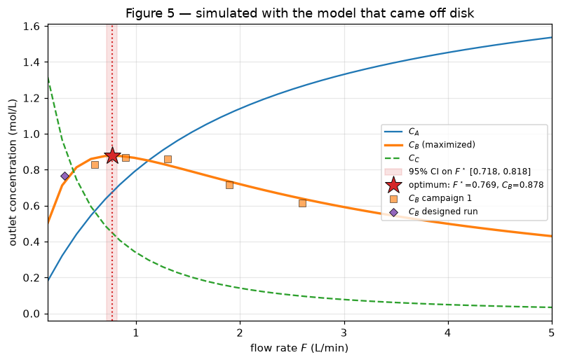
The optimum is computed from estimates, so it inherits their uncertainty. Propagating each file’s covariance through \(F^\star = V\sqrt{k_1 k_2}\) by sampling gives an honest interval on the recommended set point — and shows what the designed run bought in the units the plant actually cares about.

rng = np.random.default_rng(0)


def propagate(center, cov, size=4000):
    """95% interval on F* = V sqrt(k1 k2) implied by a calibration."""
    draws = rng.multivariate_normal(list(center), cov, size=size)
    draws = draws[(draws > 0).all(axis=1)]
    F_star = V_val * np.sqrt(draws[:, 0] * draws[:, 1])
    lo, hi = np.percentile(F_star, [2.5, 97.5])
    return float(np.mean(F_star)), float(lo), float(hi)


m1, lo1, hi1 = propagate(c1, cov1)
m2_, lo, hi = propagate(c2, cov2)
print(f"F* from {CALIBRATED_V1.name}: {m1:.4f}  [{lo1:.4f}, {hi1:.4f}]  (width {hi1 - lo1:.4f})")
print(f"F* from {CALIBRATED_V2.name}: {m2_:.4f}  [{lo:.4f}, {hi:.4f}]  (width {hi - lo:.4f})")
print(f"the designed run narrowed the recommendation by {100 * (1 - (hi - lo) / (hi1 - lo1)):.0f}%")

F* from cstr_calibrated_v1.dopt: 0.7978  [0.7292, 0.8652]  (width 0.1360)
F* from cstr_calibrated_v2.dopt: 0.7679  [0.7181, 0.8179]  (width 0.0998)
the designed run narrowed the recommendation by 27%

profile = simulate(final, theta_final["k1"], theta_final["k2"], F_dense)

fig, ax = plt.subplots(figsize=(7.4, 4.8))
ax.plot(F_dense, profile[:, 0], color="C0", label="$C_A$")
ax.plot(F_dense, profile[:, 1], color="C1", lw=2.2, label="$C_B$ (maximized)")
ax.plot(F_dense, profile[:, 2], color="C2", ls="--", label="$C_C$")

ax.axvspan(lo, hi, color="C3", alpha=0.13, label=f"95% CI on $F^\\star$ [{lo:.3f}, {hi:.3f}]")
ax.axvline(F_opt, color="C3", ls=":", lw=1.4)
ax.plot([F_opt], [CB_opt], "*", ms=17, color="C3", mec="k", mew=0.6, zorder=5,
        label=f"optimum: $F^\\star$={F_opt:.3f}, $C_B$={CB_opt:.3f}")
ax.plot(campaign["F"], campaign["CB"], "s", color="C1", mec="k", mew=0.5, alpha=0.65,
        label="$C_B$ campaign 1")
ax.plot(new_run["F"], new_run["CB"], "D", color="C4", mec="k", mew=0.5, label="$C_B$ designed run")

ax.set_xlabel("flow rate $F$ (L/min)")
ax.set_ylabel("outlet concentration (mol/L)")
ax.set_title("Figure 5 — simulated with the model that came off disk")
ax.legend(fontsize=8, loc="center right")
ax.grid(alpha=0.3)
ax.set_xlim(F_dense[0], F_dense[-1])
plt.show()

8. Open the envelope

Every number above came from the six measurements. Now, and only now, we ask cstr_lab.py what it was actually simulating.

truth = json.loads(
    subprocess.run([sys.executable, str(LAB), "--reveal"],
                   check=True, capture_output=True, text=True).stdout
)
F_true = truth["V"] * np.sqrt(truth["k1"] * truth["k2"])

rows = ["| quantity | estimated | true | error |", "|---|---:|---:|---:|"]
for i, name in enumerate(("k1", "k2")):
    est, se = theta_final[name], np.sqrt(cov2[i, i])
    rows.append(
        f"| ${name[0]}_{name[1]}$ (1/min) | {est:.4f} $\\pm$ {se:.4f} | "
        f"{truth[name]:.4f} | {est - truth[name]:+.4f} ({abs(est - truth[name]) / se:.1f}$\\sigma$) |"
    )
rows.append(
    f"| $F^\\star$ (L/min) | {F_opt:.4f} [{lo:.3f}, {hi:.3f}] | {F_true:.4f} | {F_opt - F_true:+.4f} |"
)
Markdown(
    "**Table 4 — the analysis, scored**\n\n"
    + "\n".join(rows)
    + f"\n\n*Designed flow rate: {F_next:.4f} L/min. "
    f"Information gain: det(FIM) ×{d2 / d1:.2f}. "
    f"Maximum outlet $C_B$ = {CB_opt:.4f} mol/L "
    f"({100 * CB_opt / float(fp['CA0'].value):.1f}% of the feed), "
    f"solver status `{opt.status}`, gap certified: {opt.gap_certified}.*"
)

Table 4 — the analysis, scored

| quantity | estimated | true | error | |—|—:|—:|—:| | $k_1$ (1/min) | 1.5091 $\pm$ 0.0372 | 1.5000 | +0.0091 (0.2$\sigma$) | | $k_2$ (1/min) | 0.3914 $\pm$ 0.0203 | 0.4000 | -0.0086 (0.4$\sigma$) | | $F^\star$ (L/min) | 0.7685 [0.718, 0.818] | 0.7746 | -0.0061 |

Designed flow rate: 0.3116 L/min. Information gain: det(FIM) ×2.13. Maximum outlet $C_B$ = 0.8780 mol/L (43.9% of the feed), solver status optimal, gap certified: True.

9. What to take away

One model answered four questions, and between each pair of questions it lived in a file rather than in memory:

job	free	fixed	objective	model came from
simulate	\(C_A, C_B, C_C\)	\(k_1, k_2, F\)	none (square)	build_reactor()
regress	\(k_1, k_2\)	\(F\) at each run	min weighted SSE	build_reactor(n)
design	\(F\)	\(k_1, k_2\) at \(\hat\theta\)	max \(\det \mathrm{FIM}\)	cstr_calibrated_v1.dopt
optimize	\(F\)	\(k_1, k_2\) at \(\hat\theta\)	max \(C_B\)	cstr_calibrated_v2.dopt

Three things are worth carrying away.

The free/fixed partition is the whole difference. lb == ub is how discopt says “fixed”, and Model.fixed scopes it to a block, because bounds are re-read at every solve and a stray fix would silently redefine the next problem while still reporting optimal. Nothing else about the reactor changed across the four jobs — not one equation was written twice.

A calibrated model is a deliverable, not a session. What the file carries is the model plus what the data taught us: the estimates as the start point, the Fisher information and observation count as parameters. That is enough for the next stage to design an experiment, put an interval on a recommendation, and pick up where the last one stopped — which is what makes the design in §6 sequential rather than a fresh start.

The designed experiment was chosen where the model said information was, not where it was convenient to run, and one such run tightened \(k_2\) more than a sixth point in the range already covered would have — the standard MBDoE result [Box and Lucas, 1959, Franceschini and Macchietto, 2008]. Note that “where the information is” was an interior optimum, not the extreme of the range: the criterion answered a question that eyeballing the residuals would not have. And the optimum inherits the parameters’ uncertainty, so reporting \(F^\star\) without the interval in Figure 5 would overstate what six measurements support [Bard, 1974].

The loop here was run one round by hand to keep each step visible. discopt.doe.sequential_doe automates the cycle when you can hand it a callable that runs an experiment. For the file format itself — what round-trips, what it refuses to write, and the provenance block — see Saving and loading models.

Full citation details for the works above are on the references page.