Atom projected density of states#
One major disadvantage of a planewave basis set is that it is difficult to relate the completely delocalized planewaves to localized phenomena such as bonding. Much insight into bonding has been gained by atomic/molecular orbital theory, which has carried over to the solid-state arena cite:RevModPhys.60.601. Consequently, several schemes have been developed to project the one-electron Kohn-Sham wave functions onto atomic wave functions cite:sanchez-portal1995:projec,segall1996:popul,segall1996:popul-mp. In VASP, the one electron wave functions can be projected onto spherical harmonic orbitals. The radial component of the atomic orbitals extends to infinity. In a solid, this means that the projection on one atom may overlap with the projection on a neighboring atom, resulting in double counting of electrons. Consequently, a cutoff radius was introduced, beyond which no contributions are included. It is not obvious what the best cutoff radius is. If the radius is too small, it might not capture all of the electrons associated with the atom. However, if it is too large, it may include electrons from neighboring atoms. One might want to use different cutoff radii for different atoms, which have different sizes. Furthermore, the ideal cutoff radius for an atom may change in different environments, thus it would require an iterative procedure to determine it. This difficulty arises because the orbital-band occupations are not observable, thus how the electrons are divided up between atoms is arbitrary and, as will be seen later, is sensitive to the cutoff radius (and in other DFT implementations, the basis set). However, Mulliken orbital populations have been used successfully for many years to examine the qualitative differences between similar systems, and that is precisely what these quantities are used for here. Thus, a discussion of the analysis and results is warranted.
The s and p states in a metal are typically delocalized in space and more like free-electrons, whereas the d-orbitals are fairly localized in space and have been treated successfully with tight-binding theories such as extended H"u ckel theory cite:RevModPhys.60.601, and linear muffin tin orbital theory cite:ruban1997:surfac. Consequently, the remaining discussion will be focused on the properties of the projected d-states.
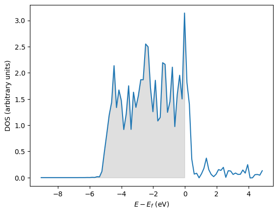
In this example, we consider how to get the atom-projected density of states (ADOS). We are interested in properties of the \(d\)-band on Pd, such as the \(d\)-band center and \(d\)-band width. You must set the [BROKEN LINK: incar:RWIGS] tag to get ADOS, and these are the Wigner-Seitz radii for each atom. By integrating the projected d-band up to the Fermi level, the d-band filling can be determined. It is not obvious what the electron count in the d-band should be for an atom in a metal. For a gas-phase, neutral metal atom in the ground state, however, the d-orbital electron count is well defined, so it will be used as an initial reference point for comparison cite:kittel.
A powerful method for characterizing distributions is to examine various moments of the distribution (see Chapter 4 in Ref. citealp:cottrell1988 and Chapter 6 in Refs. citealp:ducastelle1991 and citealp:pettifor1992:elect-theor-alloy-desig). The \(n^{th}\) order moment, \(\mu_n\), of a distribution of states \(\rho(\epsilon)\) with respect to a reference \(\epsilon_o\) is defined by
In this work, the reference energy is always the Fermi level. The zeroth moment is just the total number of states, in this case it will be normalized to unity. The first moment is the average energy of distribution, analogous to the center of mass for a mass density distribution. The second moment is the mean squared width of the distribution. The third moment is a measure of skewness and the fourth moment is related to kurtosis, but these moments are rarely used, and only the first and second moments are considered in this work.
It is important to note that these projected density of states are not physical observables. They are the wavefunctions projected onto atomic orbitals. For some situations this makes sense, e.g. the \(d\) orbitals are fairly localized and reasonably approximated by atomic orbitals. The \(s\) valence orbitals in a metal, in contrast, are almost totally delocalized. Depending on the cutoff radius (RWIGS) you choose, you can see very different ADOS.
from ase import Atoms, Atom
from vasp import Vasp

import matplotlib.pyplot as plt
import numpy as np

a = 3.9  # approximate lattice constant
b = a / 2.
bulk = Atoms([Atom('Pd', (0.0, 0.0, 0.0))],
             cell=[(0, b, b),
                   (b, 0, b),
                   (b, b, 0)])

calc = Vasp(label='bulk/pd-ados',
            encut=300,
            xc='PBE',
            lreal=False,
            rwigs={'Pd': 1.5},  # wigner-seitz radii for ados
            kpts=(8, 8, 8),
            atoms=bulk)

# this runs the calculation
calc.calculate()

# now get results
energies, ados = calc.get_ados(0, 'd')

# we will select energies in the range of -10, 5
ind = (energies < 5) & (energies > -10)

energies = energies[ind]
dos = ados[ind]

Nstates = np.trapz(dos, energies)
occupied = energies <= 0.0
N_occupied_states = np.trapz(dos[occupied], energies[occupied])
# first moment
ed = np.trapz(energies * dos, energies) / Nstates

# second moment
wd2 = np.trapz(energies**2 * dos, energies) / Nstates

print(f'Total # states = {Nstates:1.2f}')
print(f'number of occupied states = {N_occupied_states:1.2f}')
print(f'd-band center = {ed:1.2f} eV')
print(f'd-band width  = {np.sqrt(wd2):1.2f} eV')

# plot the d-band
plt.plot(energies, dos, label='$d$-orbitals')

# plot the occupied states in shaded gray
plt.fill_between(x=energies[occupied],
                 y1=dos[occupied],
                 y2=np.zeros(dos[occupied].shape),
                 color='gray', alpha=0.25)

plt.xlabel('$E - E_f$ (eV)')
plt.ylabel('DOS (arbitrary units)')
Total # states = 9.27
number of occupied states = 8.06
d-band center = -1.98 eV
d-band width  = 2.69 eV
Text(0, 0.5, 'DOS (arbitrary units)')
Effect of RWIGS on ADOS#
Here we examine the effect of changing RWIGS on the number of counted electrons, and properties of the d-band moments.
from ase import Atoms, Atom
from vasp import Vasp

import matplotlib.pyplot as plt
import numpy as np

a = 3.9  # approximate lattice constant
b = a / 2.
bulk = Atoms([Atom('Pd', (0.0, 0.0, 0.0))],
             cell=[(0, b, b),
                   (b, 0, b),
                   (b, b, 0)])

RWIGS = [1.0, 1.1, 1.25, 1.5, 2.0, 2.5, 3.0, 4.0, 5.0 ]

ED, WD, N = [], [], []

for rwigs in RWIGS:
    calc = Vasp(label='bulk/pd-ados').clone(f'bulk/pd-ados-rwigs-{rwigs}')
    calc.set(rwigs={'Pd': rwigs})
    calc.calculate()

    # now get results using calc.get_ados()
    energies, dos = calc.get_ados(0, 'd')

    # we will select energies in the range of -10, 5
    ind = (energies < 5) & (energies > -10)

    energies = energies[ind]
    dos = dos[ind]

    Nstates = np.trapz(dos, energies)
    occupied = energies <= 0.0
    N_occupied_states = np.trapz(dos[occupied], energies[occupied])
    ed = np.trapz(energies * dos, energies) / np.trapz(dos, energies)
    wd2 = np.trapz(energies**2 * dos, energies) / np.trapz(dos, energies)

    N.append(N_occupied_states)
    ED.append(ed)
    WD.append(wd2**0.5)

plt.plot(RWIGS, N, 'bo', label='N. occupied states')
plt.legend(loc='best')
plt.xlabel('RWIGS ($\AA$)')
plt.ylabel('# occupied states')


fig, ax1 = plt.subplots()
ax1.plot(RWIGS, ED, 'bo', label='d-band center (eV)')
ax1.set_xlabel('RWIGS ($\AA$)')
ax1.set_ylabel('d-band center (eV)', color='b')
for tl in ax1.get_yticklabels():
    tl.set_color('b')

ax2 = ax1.twinx()
ax2.plot(RWIGS, WD, 'gs', label='d-band width (eV)')
ax2.set_ylabel('d-band width (eV)', color='g')
for tl in ax2.get_yticklabels():
    tl.set_color('g')
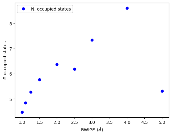
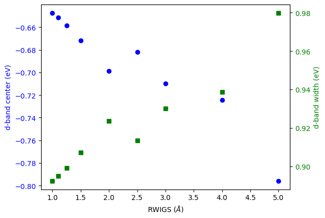
You can see the number of occupied states increases approximately linearly here with RWIGS. This is due to overcounting of neighboring electrons.
The d-band center and width also change.