Defining and visualizing molecules#
We start by learning how to define a molecule and visualize it. We will begin with defining molecules from scratch, then reading molecules from data files, and finally using some built-in databases in ase.
From scratch#
When there is no data file for the molecule you want, or no database to get it from, you have to define your atoms geometry by hand. Here is how that is done for a CO molecule (Figure ref:fig:co-origin). We must define the type and position of each atom, and the unit cell the atoms are in.
from ase import Atoms, Atom
from ase.io import write

# define an Atoms object
atoms = Atoms([Atom('C', [0., 0., 0.]),
               Atom('O', [1.1, 0., 0.])],
              cell=(10, 10, 10))

print('V = {0:1.0f} Angstrom^3'.format(atoms.get_volume()))

write('images/simple-cubic-cell.png', atoms, show_unit_cell=2)
V = 1000 Angstrom^3
V = 1000 Angstrom^3
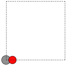
There are two inconvenient features of the simple cubic cell:
Since the CO molecule is at the corner, its electron density is spread over the 8 corners of the box, which is not convenient for visualization later (see [BROKEN LINK: *Visualizing%20electron%20density]).
Due to the geometry of the cube, you need fairly large cubes to make sure the electron density of the molecule does not overlap with that of its images. Electron-electron interactions are repulsive, and the overlap makes the energy increase significantly. Here, the CO molecule has 6 images due to periodic boundary conditions that are 10 Å away. The volume of the unit cell is 1000 Å\(^3\).
The first problem is easily solved by centering the atoms in the unit cell. The second problem can be solved by using a face-centered cubic lattice, which is the lattice with the closest packing. We show the results of the centering in Figure ref:fig:co-fcc, where we have guessed values for \(b\) until the CO molecules are on average 10 Å apart. Note the final volume is only about 715 Å\(^3\), which is smaller than the cube. This will result in less computational time to compute properties.
from ase import Atoms, Atom
from ase.io import write

b = 7.1
atoms = Atoms([Atom('C', [0., 0., 0.]),
               Atom('O', [1.1, 0., 0.])],
              cell=[[b, b, 0.],
                    [b, 0., b],
                    [0., b, b]])

print('V = {0:1.0f} Ang^3'.format(atoms.get_volume()))

atoms.center()  # translate atoms to center of unit cell
write('images/fcc-cell.png', atoms, show_unit_cell=2)
V = 716 Ang^3
V = 716 Ang^3
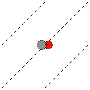
At this point you might ask, “How do you know the distance to the neighboring image?” The ag viewer lets you compute this graphically, but we can use code to determine this too. All we have to do is figure out the length of each lattice vector, because these are what separate the atoms in the images. We use the mod:numpy module to compute the distance of a vector as the square root of the sum of squared elements.
from ase import Atoms, Atom
import numpy as np

b = 7.1
atoms = Atoms([Atom('C', [0., 0., 0.]),
               Atom('O', [1.1, 0., 0.])],
              cell=[[b, b, 0.],
                    [b, 0., b],
                    [0., b, b]])

# get unit cell vectors and their lengths
(a1, a2, a3) = atoms.get_cell()
print('|a1| = {0:1.2f} Ang'.format(np.sum(a1**2)**0.5))
print('|a2| = {0:1.2f} Ang'.format(np.linalg.norm(a2)))
print('|a3| = {0:1.2f} Ang'.format(np.sum(a3**2)**0.5))
|a1| = 10.04 Ang
|a2| = 10.04 Ang
|a3| = 10.04 Ang
|a1| = 10.04 Ang
|a2| = 10.04 Ang
|a3| = 10.04 Ang
Reading other data formats into a calculation#
mod:ase.io.read supports many different file formats:
Known formats:

=========================  ===========
format                     short name
=========================  ===========
GPAW restart-file          gpw
Dacapo netCDF output file  dacapo
Old ASE netCDF trajectory  nc
Virtual Nano Lab file      vnl
ASE pickle trajectory      traj
ASE bundle trajectory      bundle
GPAW text output           gpaw-text
CUBE file                  cube
XCrySDen Structure File    xsf
Dacapo text output         dacapo-text
XYZ-file                   xyz
VASP POSCAR/CONTCAR file   vasp
VASP OUTCAR file           vasp_out
SIESTA STRUCT file         struct_out
ABINIT input file          abinit
V_Sim ascii file           v_sim
Protein Data Bank          pdb
CIF-file                   cif
FHI-aims geometry file     aims
FHI-aims output file       aims_out
VTK XML Image Data         vti
VTK XML Structured Grid    vts
VTK XML Unstructured Grid  vtu
TURBOMOLE coord file       tmol
TURBOMOLE gradient file    tmol-gradient
exciting input             exi
AtomEye configuration      cfg
WIEN2k structure file      struct
DftbPlus input file        dftb
CASTEP geom file           cell
CASTEP output file         castep
CASTEP trajectory file     geom
ETSF format                etsf.nc
DFTBPlus GEN format        gen
CMR db/cmr-file            db
CMR db/cmr-file            cmr
LAMMPS dump file           lammps
Gromacs coordinates        gro
=========================  ===========
You can read XYZ file format to create mod:ase.Atoms objects. Here is what an XYZ file format might look like:
#+include: molecules/isobutane.xyz
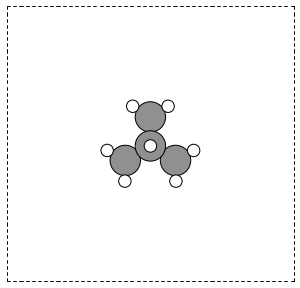
The first line is the number of atoms in the file. The second line is often a comment. What follows is one line per atom with the symbol and Cartesian coordinates in Å. Note that the XYZ format does not have unit cell information in it, so you will have to figure out a way to provide it. In this example, we center the atoms in a box with vacuum on all sides (Figure ref:fig:isobutane).
from ase.io import read, write

atoms = read('molecules/isobutane.xyz')
atoms.center(vacuum=5)
write('images/isobutane-xyz.png', atoms, show_unit_cell=2)
Predefined molecules#
mod:ase defines a number of molecular geometries in the mod:ase.data.molecules database. For example, the database includes the molecules in the G2/97 database cite:curtiss:1063. This database contains a broad set of atoms and molecules for which good experimental data exists, making them useful for benchmarking studies. See this site for the original files.
The coordinates for the atoms in the database are MP2(full)/6-31G(d) optimized geometries. Here is a list of all the species available in mod:ase.data.g2. You may be interested in reading about some of the other databases in mod:ase.data too.
from ase.data import g2
keys = list(g2.data.keys())
# print in 3 columns
for i in range(len(keys) // 3):
    print('{0:25s}{1:25s}{2:25s}'.format(*tuple(keys[i * 3: i * 3 + 3])))
Be                       BeH                      C
C2H2                     C2H4                     C2H6
CH                       CH2_s1A1d                CH2_s3B1d
CH3                      CH3Cl                    CH3OH
CH3SH                    CH4                      CN
CO                       CO2                      CS
Cl                       Cl2                      ClF
ClO                      F                        F2
H                        H2CO                     H2O
H2O2                     HCN                      HCO
HCl                      HF                       HOCl
Li                       Li2                      LiF
LiH                      N                        N2
N2H4                     NH                       NH2
NH3                      NO                       Na
Na2                      NaCl                     O
O2                       OH                       P
P2                       PH2                      PH3
S                        S2                       SH2
SO                       SO2                      Si
Si2                      Si2H6                    SiH2_s1A1d
SiH2_s3B1d               SiH3                     SiH4
SiO                      2-butyne                 Al
AlCl3                    AlF3                     B
BCl3                     BF3                      C2Cl4
C2F4                     C2H3                     C2H5
C2H6CHOH                 C2H6NH                   C2H6SO
C3H4_C2v                 C3H4_C3v                 C3H4_D2d
C3H6_Cs                  C3H6_D3h                 C3H7
C3H7Cl                   C3H8                     C3H9C
C3H9N                    C4H4NH                   C4H4O
C4H4S                    C5H5N                    C5H8
C6H6                     CCH                      CCl4
CF3CN                    CF4                      CH2NHCH2
CH2OCH2                  CH2SCH2                  CH3CH2Cl
CH3CH2NH2                CH3CH2O                  CH3CH2OCH3
CH3CH2OH                 CH3CH2SH                 CH3CHO
CH3CN                    CH3CO                    CH3COCH3
CH3COCl                  CH3COF                   CH3CONH2
CH3COOH                  CH3NO2                   CH3O
CH3OCH3                  CH3ONO                   CH3S
CH3SCH3                  CH3SiH3                  COF2
CS2                      ClF3                     ClNO
F2O                      H2                       H2CCHCN
H2CCHCl                  H2CCHF                   H2CCO
H2CCl2                   H2CF2                    H2COH
H3CNH2                   HCCl3                    HCF3
HCOOCH3                  HCOOH                    N2O
NCCN                     NF3                      NO2
O3                       OCHCHO                   OCS
PF3                      SH                       SiCl4
SiF4                     bicyclobutane            butadiene
cyclobutane              cyclobutene              isobutane
isobutene                methylenecyclopropane    trans-butane
Some other databases include the mod:ase.data.s22 for weakly interacting dimers and complexes, and mod:ase.data.extramolecules which has a few extras like biphenyl and C60.
Here is an example of getting the geometry of an acetonitrile molecule and writing an image to a file. Note that the default unit cell is a 1 Å × Å × Å cubic cell. That is too small to use if your calculator uses periodic boundary conditions. We center the atoms in the unit cell and add vacuum on each side. We will add 6 Å of vacuum on each side. In the write command we use the option show_unit_cell =2 to draw the unit cell boundaries. See Figure ref:fig:ch3cn.
from ase.build import molecule
from ase.io import write


atoms = molecule('CH3CN')

atoms.center(vacuum=6)
print('unit cell')
print('---------')
print(atoms.get_cell())

write('images/ch3cn.png', atoms, show_unit_cell=2)
unit cell
---------
Cell([13.775328, 13.537479, 15.014576])
from ase.build import molecule
from ase.io import write

atoms = molecule('CH3CN')

atoms.center(vacuum=6)
print('unit cell')
print('---------')
print(atoms.get_cell())

write('images/ch3cn-rotated.png', atoms,
      show_unit_cell=2, rotation='45x,45y,0z')
unit cell
---------
Cell([13.775328, 13.537479, 15.014576])
from ase.build import molecule
from ase.io import write
from numpy import pi

atoms = molecule('CH3CN')
atoms.center(vacuum=6)
p1 = atoms.get_positions()

atoms.rotate('x', pi/4, center='COM', rotate_cell=False)
atoms.rotate('y', pi/4, center='COM', rotate_cell=False)

write('images/ch3cn-rotated-2.png', atoms, show_unit_cell=2)
print('difference in positions after rotating')
print('atom    difference vector')
print('--------------------------------------')
p2 = atoms.get_positions()

diff = p2 - p1
for i, d in enumerate(diff):
    print('{0} {1}'.format(i, d))
difference in positions after rotating
atom    difference vector
--------------------------------------
0 [-0.01782051  0.01782219  0.0002443 ]
1 [ 2.20136479e-03 -2.20157163e-03 -3.01777230e-05]
2 [ 0.01835166 -0.01835339 -0.00025158]
3 [-0.02277373  0.02287218  0.01436336]
4 [-0.02314601  0.02301662 -0.01887695]
5 [-0.02297922  0.02301662  0.0054581 ]
Combining Atoms objects#
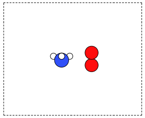
It is frequently useful to combine two Atoms objects, e.g. for computing reaction barriers, or other types of interactions. In ase, we simply add two Atoms objects together. Here is an example of getting an ammonia and oxygen molecule in the same unit cell. See Figure ref:fig:combined-atoms. We set the Atoms about three Å apart using the func:ase.Atoms.translate function.
from ase.build import molecule
from ase.io import write

atoms1 = molecule('NH3')

atoms2 = molecule('O2')
atoms2.translate([3, 0, 0])

bothatoms = atoms1 + atoms2
bothatoms.center(5)

write('images/bothatoms.png', bothatoms, show_unit_cell=2, rotation='90x')