Running Aspen via Python

| categories: programming | tags: aspen

Aspen is a process modeling tool that simulates industrial processes. It has a GUI for setting up the flowsheet, defining all the stream inputs and outputs, and for running the simulation. For single calculations it is pretty convenient. For many calculations, all the pointing and clicking to change properties can be tedious, and difficult to reproduce. Here we show how to use Python to automate Aspen using the COM interface.

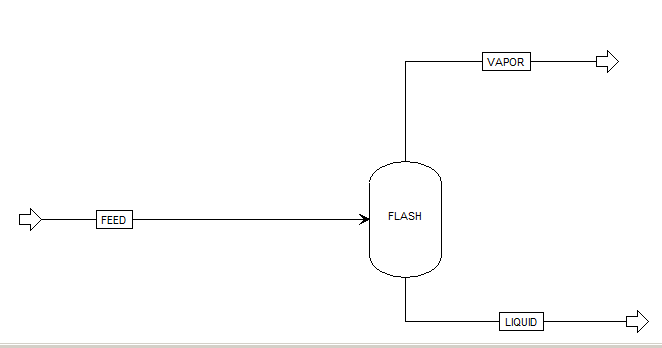
We have an Aspen flowsheet setup for a flash operation. The feed consists of 91.095 mol% water and 8.905 mol% ethanol at 100 degF and 50 psia. 48.7488 lbmol/hr of the mixture is fed to the flash tank which is at 150 degF and 20 psia. We want to know the composition of the VAPOR and LIQUID streams. The simulation has been run once.

This is an example that just illustrates it is possible to access data from a simulation that has been run. You have to know quite a bit about the Aspen flowsheet before writing this code. Particularly, you need to open the Variable Explorer to find the "path" to the variables that you want, and to know what the units are of those variables are.

import os
import win32com.client as win32
aspen = win32.Dispatch('Apwn.Document')

aspen.InitFromArchive2(os.path.abspath('data\Flash_Example.bkp'))

## Input variables
feed_temp = aspen.Tree.FindNode('\Data\Streams\FEED\Input\TEMP\MIXED').Value
print 'Feed temperature was {0} degF'.format(feed_temp)

ftemp = aspen.Tree.FindNode('\Data\Blocks\FLASH\Input\TEMP').Value
print 'Flash temperature = {0}'.format(ftemp)

## Output variables
eL_out = aspen.Tree.FindNode("\Data\Streams\LIQUID\Output\MOLEFLOW\MIXED\ETHANOL").Value
wL_out = aspen.Tree.FindNode("\Data\Streams\LIQUID\Output\MOLEFLOW\MIXED\WATER").Value

eV_out = aspen.Tree.FindNode("\Data\Streams\VAPOR\Output\MOLEFLOW\MIXED\ETHANOL").Value
wV_out = aspen.Tree.FindNode("\Data\Streams\VAPOR\Output\MOLEFLOW\MIXED\WATER").Value

tot = aspen.Tree.FindNode("\Data\Streams\FEED\Input\TOTFLOW\MIXED").Value

print 'Ethanol vapor mol flow: {0} lbmol/hr'.format(eV_out)
print 'Ethanol liquid mol flow: {0} lbmol/hr'.format(eL_out)

print 'Water vapor mol flow: {0} lbmol/hr'.format(wV_out)
print 'Water liquid mol flow: {0} lbmol/hr'.format(wL_out)

print 'Total = {0}. Total in = {1}'.format(eV_out + eL_out + wV_out + wL_out,
                                           tot)

aspen.Close()
Feed temperature was 100.0 degF
Flash temperature = 150.0
Ethanol vapor mol flow: 3.89668323 lbmol/hr
Ethanol liquid mol flow: 0.444397241 lbmol/hr
Water vapor mol flow: 0.774592763 lbmol/hr
Water liquid mol flow: 43.6331268 lbmol/hr
Total = 48.748800034. Total in = 48.7488

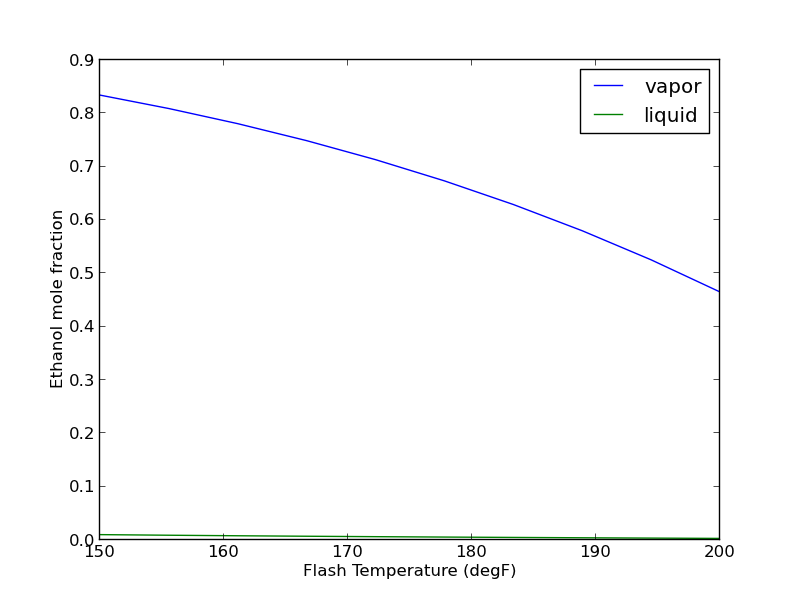
It is nice that we can read data from a simulation, but it would be helpful if we could change variable values and to rerun the simulations. That is possible. We simply set the value of the variable, and tell Aspen to rerun. Here, we will change the temperature of the Flash tank and plot the composition of the outlet streams as a function of that temperature.

import os
import numpy as np
import matplotlib.pyplot as plt
import win32com.client as win32

aspen = win32.Dispatch('Apwn.Document')
aspen.InitFromArchive2(os.path.abspath('data\Flash_Example.bkp'))

T = np.linspace(150, 200, 10)

x_ethanol, y_ethanol = [], []

for temperature in T:
    aspen.Tree.FindNode('\Data\Blocks\FLASH\Input\TEMP').Value = temperature
    aspen.Engine.Run2()

    x_ethanol.append(aspen.Tree.FindNode('\Data\Streams\LIQUID\Output\MOLEFRAC\MIXED\ETHANOL').Value)
    y_ethanol.append(aspen.Tree.FindNode('\Data\Streams\VAPOR\Output\MOLEFRAC\MIXED\ETHANOL').Value)

plt.plot(T, y_ethanol, T, x_ethanol)
plt.legend(['vapor', 'liquid'])
plt.xlabel('Flash Temperature (degF)')
plt.ylabel('Ethanol mole fraction')
plt.savefig('images/aspen-water-ethanol-flash.png')
aspen.Close()

It takes about 30 seconds to run the previous example. Unfortunately, the way it is written, if you want to change anything, you have to run all of the calculations over again. How to avoid that is moderately tricky, and will be the subject of another example.

In summary, it seems possible to do a lot with Aspen automation via python. This can also be done with Matlab, Excel, and other programming languages where COM automation is possible. The COM interface is not especially well documented, and you have to do a lot of digging to figure out some things. It is not clear how committed Aspen is to maintaining or improving the COM interface (http://www.chejunkie.com/aspen-plus/aspen-plus-activex-automation-server/). Hopefully they can keep it alive for power users who do not want to program in Excel!

Copyright (C) 2013 by John Kitchin. See the License for information about copying.

org-mode source

Discuss on Twitter

Reading and writing pdf metadata

| categories: programming | tags:

One key to automating analysis of files is that data be stored in files in a way that is easy to add and retrieve. I have been examining ways to add grades to files so that a program could read the file, extract the grade, and collect it in a gradebook.

PDF files could be one format where this is possible. The idea is that students would turn in a PDF file as their homework. The assignment would be graded, perhaps with hand-written markup from a tablet, and the grader would enter the grade as custom metadata in the file. Later a program would read the grade in and compile the results.

In this post I examine some python modules that can do this. There are several python modules that can interact with PDF files.

  1. pyPDF (seems to be replaced by PyPDF2).
  2. pdfrw
  3. pdfMiner (seems to be read-only)

All of these can be installed with pip. First, we look at getting existing information from a PDF file.

from pyPdf import PdfFileReader, PdfFileWriter

fname = '../../../Desktop/Program Organizer Controls.pdf'

pdf = PdfFileReader(open(fname, 'rb'))

print pdf.getDocumentInfo()
{'/Creator': u'Bluebeam Stapler 10.2.1', '/Author': u'John Kitchin', '/Producer': u'Bluebeam Brewery 5.0', '/CreationDate': u"D:20130612143804-04'00'", '/ModDate': u"D:20130613095927-04'00'"}

That is pretty straightfoward. Now, let us add some new metadata. We will create a Grade metadata, and store the grade in it. It appears we need to read in the pdf file, add its pages and metadata to a writer, set the new metadata, and then write out the file.

It seems that we cannot directly modify the PDF file, so we will write out to a new file, delete the old file, and rename the new file to the old file.

from pyPdf import PdfFileReader, PdfFileWriter
from pyPdf.generic import NameObject, createStringObject

inpfn = '../../../Desktop/Program Organizer Controls.pdf'

fin = file(inpfn, 'rb')
pdf_in = PdfFileReader(fin)

writer = PdfFileWriter()

for page in range(pdf_in.getNumPages()):
    writer.addPage(pdf_in.getPage(page))

infoDict = writer._info.getObject()

info = pdf_in.documentInfo
for key in info:
    infoDict.update({NameObject(key): createStringObject(info[key])})

# add the grade
infoDict.update({NameObject('/Grade'): createStringObject(u'A+')})

# It does not appear possible to alter in place.
fout = open(inpfn+'out.pdf', 'wb')

writer.write(fout)
fin.close()
fout.close()

import os
os.unlink(inpfn)
os.rename(inpfn+'out.pdf', inpfn)

Finally, we can see we successfully modified the file.

from pyPdf import PdfFileReader, PdfFileWriter

fname = '../../../Desktop/Program Organizer Controls.pdf'

pdf = PdfFileReader(open(fname, 'rb'))

print pdf.getDocumentInfo()
print pdf.getDocumentInfo()['/Grade']
{'/Grade': u'A+', '/CreationDate': u"D:20130612143804-04'00'", '/Producer': u'Bluebeam Brewery 5.0', '/Creator': u'Bluebeam Stapler 10.2.1', '/ModDate': u"D:20130613095927-04'00'", '/Author': u'John Kitchin'}
A+

You can see we were able to successfully add a Grade metadata field. It is stored as a Custom Document Property in my PDF viewer. I am not sure how easy it would be for a grader to enter this into a PDF. It could be possible to automate this with some kind of script that made a decent workflow. For example an org-mode file could have links that open the PDF, allow you to grade it. Then, you could click on another link that would prompt you for the grade, and then add it to the pdf. Or maybe a small script could be written that would open the pdf, wait for your to close it, then prompt you for the grade before moving to the next one.

Copyright (C) 2013 by John Kitchin. See the License for information about copying.

org-mode source

Discuss on Twitter

Finding the volume of a unit cell at a fixed pressure

| categories: uncategorized | tags:

A typical unit cell optimization in DFT is performed by minimizing the total energy with respect to variations in the unit cell parameters and atomic positions. In this approach, a pressure of 0 GPa is implied, as well as a temperature of 0K. For non-zero pressures, the volume that minimizes the total energy is not the same as the volume at P=0.

Let \(x\) be the unit cell parameters that can be varied. For P ≠ 0, and T = 0, we have the following

\(G(x; p) = E(x) + p V(x)\)

and we need to minimize this function to find the groundstate volume. We will do this for fcc Cu at 5 GPa of pressure. We will assume there is only one degree of freedom in the unit cell, the lattice constant. First we get the \(E(x)\) function, and then add the analytical correction.

from jasp import *
from ase import Atom, Atoms
from ase.utils.eos import EquationOfState

LC = [3.5, 3.55, 3.6, 3.65, 3.7, 3.75]
volumes, energies = [], []
ready = True

P = 5.0 / 160.2176487  # pressure in eV/ang**3

for a in LC:
    atoms = Atoms([Atom('Cu',(0, 0, 0))],
              cell=0.5 * a*np.array([[1.0, 1.0, 0.0],
                                     [0.0, 1.0, 1.0],
                                     [1.0, 0.0, 1.0]]))

    with jasp('../bulk/Cu-{0}'.format(a),
              xc='PBE',
              encut=350,
              kpts=(8,8,8),
              atoms=atoms) as calc:

        try:
            e = atoms.get_potential_energy()
            energies.append(e)
            volumes.append(atoms.get_volume())
        except (VaspSubmitted, VaspQueued):
            ready = False

if not ready:
    import sys; sys.exit()

import numpy as np
energies = np.array(energies)
volumes = np.array(volumes)

eos = EquationOfState(volumes, energies)
v0, e0, B = eos.fit()
print 'V0 at 0 GPa = {0:1.2f} ang^3'.format(v0)

eos5 = EquationOfState(volumes, energies + P * volumes)
v0_5, e0, B = eos5.fit()
print 'V0 at 5 GPa = {0:1.2f} ang^3'.format(v0_5)
V0 at 0 GPa = 12.02 ang^3
V0 at 5 GPa = 11.62 ang^3

You can see here that apply pressure decreases the equilibrium volume, and increases the total energy.

Copyright (C) 2013 by John Kitchin. See the License for information about copying.

org-mode source

Discuss on Twitter

Constrained fits to data

| categories: data analysis, optimization | tags:

Our objective here is to fit a quadratic function in the least squares sense to some data, but we want to constrain the fit so that the function has specific values at the end-points. The application is to fit a function to the lattice constant of an alloy at different compositions. We constrain the fit because we know the lattice constant of the pure metals, which are at the end-points of the fit and we want these to be correct.

We define the alloy composition in terms of the mole fraction of one species, e.g. \(A_xB_{1-x}\). For \(x=0\), the alloy is pure B, whereas for \(x=1\) the alloy is pure A. According to Vegard's law the lattice constant is a linear composition weighted average of the pure component lattice constants, but sometimes small deviations are observed. Here we will fit a quadratic function that is constrained to give the pure metal component lattice constants at the end points.

The quadratic function is \(y = a x^2 + b x + c\). One constraint is at \(x=0\) where \(y = c\), or \(c\) is the lattice constant of pure B. The second constraint is at \(x=1\), where \(a + b + c\) is equal to the lattice constant of pure A. Thus, there is only one degree of freedom. \(c = LC_B\), and \(b = LC_A - c - a\), so \(a\) is our only variable.

We will solve this problem by minimizing the summed squared error between the fit and the data. We use the fmin function in scipy.optimize. First we create a fit function that encodes the constraints. Then we create an objective function that will be minimized. We have to make a guess about the value of \(a\) that minimizes the summed squared error. A line fits the data moderately well, so we guess a small value, i.e. near zero, for \(a\). Here is the solution.

import numpy as np
import matplotlib.pyplot as plt

# Data to fit to
# x=0 is pure B
# x=1 is pure A
X = np.array([0.0, 0.1,  0.25, 0.5,  0.6,  0.8,  1.0])
Y = np.array([3.9, 3.89, 3.87, 3.78, 3.75, 3.69, 3.6])

def func(a, XX):
    LC_A = 3.6
    LC_B = 3.9

    c = LC_B
    b = LC_A - c - a

    yfit = a * XX**2 + b * XX + c
    return yfit

def objective(a):
    'function to minimize'
    SSE = np.sum((Y - func(a, X))**2)
    return SSE


from scipy.optimize import fmin

a_fit = fmin(objective, 0)
plt.plot(X, Y, 'bo ')

x = np.linspace(0, 1)
plt.plot(x, func(a_fit, x))
plt.savefig('images/constrained-quadratic-fit.png')
Optimization terminated successfully.
         Current function value: 0.000445
         Iterations: 19
         Function evaluations: 38

Here is the result:

You can see that the end points go through the end-points as prescribed.

Copyright (C) 2013 by John Kitchin. See the License for information about copying.

org-mode source

Discuss on Twitter

What region is a point in

| categories: programming | tags:

Suppose we have a space that is divided by a boundary into two regions, and we want to know if an arbitrary point is on one region or the other. One way to figure this out is to pick a point that is known to be in a region, and then draw a line to the arbitrary point counting the number of times it crosses the boundary. If the line crosses an even number of times, then the point is in the same region and if it crosses an odd number of times, then the point is in the other region.

Here is the boundary and region we consider in this example:

boundary = [[0.1, 0],
            [0.25, 0.1],
            [0.3, 0.2],
            [0.35, 0.34],
            [0.4, 0.43],
            [0.51, 0.47],
            [0.48, 0.55],
            [0.44, 0.62],
            [0.5, 0.66],
            [0.55,0.57],
            [0.556, 0.48],
            [0.63, 0.43],
            [0.70, 0.44],
            [0.8, 0.51],
            [0.91, 0.57],
            [1.0, 0.6]]

import matplotlib.pyplot as plt

plt.plot([p[0] for p in boundary],
         [p[1] for p in boundary])
plt.ylim([0, 1])
plt.savefig('images/boundary-1.png')
... ... ... ... ... ... ... ... ... ... ... ... ... ... >>> >>> >>> >>> >>> ... [<matplotlib.lines.Line2D object at 0x00000000062FEBA8>]
(0, 1)

In this example, the boundary is complicated, and not described by a simple function. We will check for intersections of the line from the arbitrary point to the reference point with each segment defining the boundary. If there is an intersection in the boundary, we count that as a crossing. We choose the origin (0, 0) in this case for the reference point. For an arbitrary point (x1, y1), the equation of the line is therefore (provided x1 !=0):

\(y = \frac{y1}{x1} x\).

Let the points defining a boundary segment be (bx1, by1) and (bx2, by2). The equation for the line connecting these points (provided bx1 != bx2) is:

\(y = by1 + \frac{by2 - by1}{bx2 - bx1}(x - bx1)\)

Setting these two equations equal to each other, we can solve for the value of \(x\), and if \(bx1 <= x <= bx2\) then we would say there is an intersection with that segment. The solution for x is:

\(x = \frac{m bx1 - by1}{m - y1/x1}\)

This can only fail if \(m = y1/x1\) which means the segments are parallel and either do not intersect or go through each other. One issue we have to resolve is what to do when the intersection is at the boundary. In that case, we would see an intersection with two segments since bx1 of one segment is also bx2 of another segment. We resolve the issue by only counting intersections with bx1. Finally, there may be intersections at values of \(x\) greater than the point, and we are not interested in those because the intersections are not between the point and reference point.

Here are all of the special cases that we have to handle:

We will have to do float comparisons, so we will define tolerance functions for all of these. I tried this previously with regular comparison operators, and there were many cases that did not work because of float comparisons. In the code that follows, we define the tolerance functions, the function that handles almost all the special cases, and show that it almost always correctly identifies the region a point is in.

import numpy as np

TOLERANCE = 2 * np.spacing(1)

def feq(x, y, epsilon=TOLERANCE):
    'x == y'
    return not((x < (y - epsilon)) or (y < (x - epsilon)))

def flt(x, y, epsilon=TOLERANCE):
    'x < y'
    return x < (y - epsilon)

def fgt(x, y, epsilon=TOLERANCE):
    'x > y'
    return y < (x - epsilon)

def fle(x, y, epsilon=TOLERANCE):
    'x <= y'
    return not(y < (x - epsilon))

def fge(x, y, epsilon=TOLERANCE):
    'x >= y'
    return not(x < (y - epsilon))

boundary = [[0.1, 0],
            [0.25, 0.1],
            [0.3, 0.2],
            [0.35, 0.34],
            [0.4, 0.43],
            [0.51, 0.47],
            [0.48, 0.55],
            [0.44, 0.62],
            [0.5, 0.66],
            [0.55,0.57],
            [0.556, 0.48],
            [0.63, 0.43],
            [0.70, 0.44],
            [0.8, 0.51],
            [0.91, 0.57],
            [1.0, 0.6]]

def intersects(p, isegment):
    'p is a point (x1, y1), isegment is an integer indicating which segment starting with 0'
    x1, y1 = p
    bx1, by1 = boundary[isegment]
    bx2, by2 = boundary[isegment + 1]

    # outline cases to handle
    if feq(bx1, bx2) and feq(x1, 0.0): # both segments are vertical
        if feq(bx1, x1):
            return True
        else:
            return False
    elif feq(bx1, bx2):  # segment is vertical
        m1 = y1 / x1 # slope of reference line
        y = m1 * bx1 # value of reference line at bx1
        if ((fge(y, by1) and flt(y, by2))
            or (fle(y, by1) and fgt(y,by2))):
            # reference line intersects the segment
            return True
        else:
            return False
    else: # neither reference line nor segment is vertical
        m = (by2 - by1) / (bx2 - bx1) # segment slope
        m1 = y1 / x1
        if feq(m, m1): # line and segment are parallel
            if feq(y1, m * bx1):
                return True
            else:
                return False
        else: # lines are not parallel
            x = (m * bx1 - by1) / (m - m1) # x at intersection

            if ((fge(x, bx1) and flt(x, bx2))
                or (fle(x, bx1) and fgt(x, bx2))) and fle(x, x1):
                return True
            else:
                return False

    raise Exception('you should not get here')

import matplotlib.pyplot as plt

plt.plot([p[0] for p in boundary],
         [p[1] for p in boundary], 'go-')
plt.ylim([0, 1])

N = 100

X = np.linspace(0, 1, N)

for x in X:
    for y in X:
        p = (x, y)
        
        nintersections = sum([intersects(p, i) for i in range(len(boundary) - 1)])

        if nintersections % 2 == 0:
            plt.plot(x, y, 'r.')
        else:
            plt.plot(x, y, 'b.')

plt.savefig('images/boundary-2.png')
plt.show()

If you look carefully, there are two blue points in the red region, which means there is some edge case we do not capture in our function. Kudos to the person who figures it out.

Copyright (C) 2013 by John Kitchin. See the License for information about copying.

org-mode source

Discuss on Twitter
« Previous Page -- Next Page »