The Kitchin Research Group

Our objective here is to fit a quadratic function in the least squares sense to some data, but we want to constrain the fit so that the function has specific values at the end-points. The application is to fit a function to the lattice constant of an alloy at different compositions. We constrain the fit because we know the lattice constant of the pure metals, which are at the end-points of the fit and we want these to be correct.

We define the alloy composition in terms of the mole fraction of one species, e.g. \(A_xB_{1-x}\). For \(x=0\), the alloy is pure B, whereas for \(x=1\) the alloy is pure A. According to Vegard's law the lattice constant is a linear composition weighted average of the pure component lattice constants, but sometimes small deviations are observed. Here we will fit a quadratic function that is constrained to give the pure metal component lattice constants at the end points.

The quadratic function is \(y = a x^2 + b x + c\). One constraint is at \(x=0\) where \(y = c\), or \(c\) is the lattice constant of pure B. The second constraint is at \(x=1\), where \(a + b + c\) is equal to the lattice constant of pure A. Thus, there is only one degree of freedom. \(c = LC_B\), and \(b = LC_A - c - a\), so \(a\) is our only variable.

We will solve this problem by minimizing the summed squared error between the fit and the data. We use the fmin function in scipy.optimize. First we create a fit function that encodes the constraints. Then we create an objective function that will be minimized. We have to make a guess about the value of \(a\) that minimizes the summed squared error. A line fits the data moderately well, so we guess a small value, i.e. near zero, for \(a\). Here is the solution.

import numpy as np
import matplotlib.pyplot as plt

# Data to fit to
# x=0 is pure B
# x=1 is pure A
X = np.array([0.0, 0.1,  0.25, 0.5,  0.6,  0.8,  1.0])
Y = np.array([3.9, 3.89, 3.87, 3.78, 3.75, 3.69, 3.6])

def func(a, XX):
    LC_A = 3.6
    LC_B = 3.9

    c = LC_B
    b = LC_A - c - a

    yfit = a * XX**2 + b * XX + c
    return yfit

def objective(a):
    'function to minimize'
    SSE = np.sum((Y - func(a, X))**2)
    return SSE


from scipy.optimize import fmin

a_fit = fmin(objective, 0)
plt.plot(X, Y, 'bo ')

x = np.linspace(0, 1)
plt.plot(x, func(a_fit, x))
plt.savefig('images/constrained-quadratic-fit.png')

Optimization terminated successfully.
         Current function value: 0.000445
         Iterations: 19
         Function evaluations: 38

Here is the result:

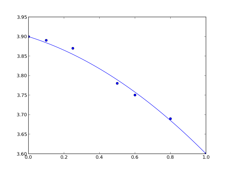
You can see that the end points go through the end-points as prescribed.

Copyright (C) 2013 by John Kitchin. See the License for information about copying.

org-mode source