The Kitchin Research Group

In high-throughput calculations, some fraction of them usually fail for some reason. Sometimes it is easy to fix these calculations and re-run them successfully, for example, you might just need a different initialization, or to increase memory or the number of allowed steps, etc. custodian is a tool that is designed for this purpose.

The idea is we make a function to do what we want that has arguments that control that. We need a function that can examine the output of the function and determine if it succeeded, and if it didn't succeed to say what new arguments to try next. Then we run the function in custodian and let it take care of rerunning with new arguments until it either succeeds, or tries too many times.

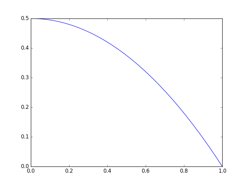
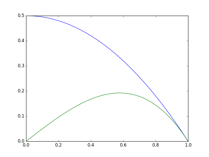
The goal here is to use custodian to fix a problem optimization. The example is a little contrived, we set a number of iterations artificially low so that the minimization fails by reaching the maximum number of iterations. Custodian will catch this, and increase the number of iterations until it succeeds. Here is the objective function:

import matplotlib.pyplot as plt
import numpy as np

def objective(x):
    return np.exp(x**2) - 10*np.exp(x)

x = np.linspace(0, 2)
plt.plot(x, objective(x))
plt.xlabel('x')
plt.ylabel('y');

Clearly there is a minimum near 1.75, but with a bad initial guess, and not enough iterations, an optimizer fails here. We can tell it fails from the message here, and the solution is run it again with more iterations.

from scipy.optimize import minimize

minimize(objective, 0.0, options={'maxiter': 2})

:RESULTS:
  message: Maximum number of iterations has been exceeded.
  success: False
   status: 1
      fun: -36.86289091418059
        x: [ 1.661e+00]
      nit: 2
      jac: [-2.374e-01]
 hess_inv: [[ 6.889e-03]]
     nfev: 20
     njev: 10
:END:

With Custodian you define a "Job". This is a class with params that contain the adjustable arguments in a dictionary, and a run method that stores the results in the params attribute. This is an important step, because the error handlers only get the params, so you need the results in there to inspect them.

The error handlers are another class with a check method that returns True if you should rerun, and a correct method that sets the params to new values to try next. It seems to return some information about what happened. In the correct method, we double the maximum number of iterations allowed, and use the last solution point that failed as the initial guess for the next run.

from custodian.custodian import Custodian, Job, ErrorHandler

class Minimizer(Job):
    def __init__(self, params=None):
        self.params = params if params else {'maxiter': 2, 'x0': 0}
        
    def run(self):
        sol = minimize(objective,
                       self.params['x0'],
                       options={'maxiter': self.params['maxiter']})
        self.params['sol'] = sol

class MaximumIterationsExceeded(ErrorHandler):
    def __init__(self, params):
        self.params = params

    def check(self):
        return self.params['sol'].message == 'Maximum number of iterations has been exceeded.'

    def correct(self):
        self.params['maxiter'] *= 2
        self.params['x0'] = self.params['sol'].x        
        return {'errors': 'MaximumIterations Exceeded',
                'actions': 'maxiter = {self.params["maxiter"]}, x0 = {self.params["x0"]}'}

Now we setup the initial params to try, create a Custodian object with the handler and job, and then run it. The results and final params are stored in the params object.

params = {'maxiter': 1, 'x0': 0}

c = Custodian([MaximumIterationsExceeded(params)],
              [Minimizer(params)],
               max_errors=5)

c.run()
for key in params:
    print(key, params[key])

MaximumIterationsExceeded
MaximumIterationsExceeded
maxiter 4
x0 [1.66250127]
sol   message: Optimization terminated successfully.
  success: True
   status: 0
      fun: -36.86307468296398
        x: [ 1.662e+00]
      nit: 1
      jac: [-9.060e-06]
 hess_inv: [[1]]
     nfev: 6
     njev: 3

Note that params is modified, and finally has the maxiter value that worked, and the solution in it. You can see we had to rerun this problem twice before it succeeded, but this happened automatically after the setup. This example is easy because we can simply increase the maxiter value, and no serious logic is needed. Other use cases might include try it again with another solver, try again with a different initial guess, etc.

It feels a little heavyweight to define the classes, and to store the results in params here, but this was overall under an hour of work to put it all together, starting from scratch with the Custodian documentation from the example on the front page. You can do more sophisticated things, including having multiple error handlers. Overall, for a package designed for molecular simulations, this worked well for a different kind of problem.

Copyright (C) 2023 by John Kitchin. See the License for information about copying.

org-mode source

Org-mode version = 9.7-pre

Almost 10 years ago I wrote about finding the minimum distance from a point to a curve using a constrained optimization. At that time, the way to do this used scipy.optimize.fmin_coblya. I learned today from a student, that sometimes this method fails! I reproduce the code here, updated for Python 3, some style updates, and to show it does indeed fail sometimes, notably when the point is "outside" the parabola.

import numpy as np
import matplotlib.pyplot as plt
from scipy.optimize import fmin_cobyla

def f(x):
    return x**2

for P in np.array([[0.5, 2],
                   [2, 2],
                   [-1, 2],
                   [-2, 2],
                   [0, 0.5],
                   [0, -0.5]]):
    
    def objective(X):
        X = np.array(X)
        return np.linalg.norm(X - P)

    def c1(X):
        x,y = X
        return f(x) - y

    X = fmin_cobyla(objective, x0=[P[0], f(P[0])], cons=[c1])

    print(f'The minimum distance is {objective(X):1.2f}. Constraint satisfied = {c1(X) < 1e-6}')

    # Verify the vector to this point is normal to the tangent of the curve
    # position vector from curve to point
    v1 = np.array(P) - np.array(X)
    # position vector
    v2 = np.array([1, 2.0 * X[0]])
    print('dot(v1, v2) = ', np.dot(v1, v2))

    x = np.linspace(-2, 2, 100)

    plt.plot(x, f(x), 'r-', label='f(x)')
    plt.plot(P[0], P[1], 'bo', label='point')
    plt.plot([P[0], X[0]], [P[1], X[1]], 'b-', label='shortest distance')
    plt.plot([X[0], X[0] + 1], [X[1], X[1] + 2.0 * X[0]], 'g-', label='tangent')
    plt.axis('equal')
    plt.xlabel('x')
    plt.ylabel('y')    

The minimum distance is 0.86. Constraint satisfied = True dot(v1, v2) = 0.0002913487659186309 The minimum distance is 0.00. Constraint satisfied = False dot(v1, v2) = 0.00021460906432962284 The minimum distance is 0.39. Constraint satisfied = True dot(v1, v2) = 0.00014271520451364372 The minimum distance is 0.00. Constraint satisfied = False dot(v1, v2) = -0.0004089466778209598 The minimum distance is 0.50. Constraint satisfied = True dot(v1, v2) = 1.9999998429305957e-12 The minimum distance is 0.00. Constraint satisfied = False dot(v1, v2) = 8.588744170160093e-06

So, sure enough, the optimizer is failing to find a solution that meets the constraint. It is strange it does not work on the outside. That is almost certainly an algorithm problem. Here we solve it nearly identically with the more modern scipy.optimize.minimize function, and it converges every time.

from scipy.optimize import minimize

for P in np.array([[0.5, 2],
                   [2, 2],
                   [-1, 2],
                   [-2, 2],
                   [0, 0.5],
                   [0, -0.5]]):
    
    def objective(X):
        X = np.array(X)
        return np.linalg.norm(X - P)

    def c1(X):
        x,y = X
        return f(x) - y

    sol = minimize(objective, x0=[P[0], f(P[0])], constraints={'type': 'eq', 'fun': c1})
    X = sol.x

    print(f'The minimum distance is {objective(X):1.2f}. Constraint satisfied = {sol.status < 1e-6}')

    # Verify the vector to this point is normal to the tangent of the curve
    # position vector from curve to point
    v1 = np.array(P) - np.array(X)
    # position vector
    v2 = np.array([1, 2.0 * X[0]])
    print('dot(v1, v2) = ', np.dot(v1, v2))

    x = np.linspace(-2, 2, 100)

    plt.plot(x, f(x), 'r-', label='f(x)')
    plt.plot(P[0], P[1], 'bo', label='point')
    plt.plot([P[0], X[0]], [P[1], X[1]], 'b-', label='shortest distance')
    plt.plot([X[0], X[0] + 1], [X[1], X[1] + 2.0 * X[0]], 'g-', label='tangent')
    plt.axis('equal')
    plt.xlabel('x')
    plt.ylabel('y')

The minimum distance is 0.86. Constraint satisfied = True dot(v1, v2) = 1.0701251773603815e-08 The minimum distance is 0.55. Constraint satisfied = True dot(v1, v2) = -0.0005793028003104883 The minimum distance is 0.39. Constraint satisfied = True dot(v1, v2) = -1.869272921939391e-05 The minimum distance is 0.55. Constraint satisfied = True dot(v1, v2) = 0.0005792953298950909 The minimum distance is 0.50. Constraint satisfied = True dot(v1, v2) = 0.0 The minimum distance is 0.50. Constraint satisfied = True dot(v1, v2) = 0.0

There is no wisdom in fixing the first problem, here I just tried a newer optimization method. Out of the box with default settings it just worked. I did learn the answer is sensitive to the initial guess, so it could make sense to sample the function and find the point that is closest as the initial guess, but here the simple heuristic guess I used worked fine.

Copyright (C) 2023 by John Kitchin. See the License for information about copying.

org-mode source

Org-mode version = 9.5.5

Constrained optimization is common in engineering problems solving. A prototypical example (from Greenberg, Advanced Engineering Mathematics, Ch 13.7) is to find the point on a plane that is closest to the origin. The plane is defined by the equation \(2x - y + z = 3\), and we seek to minimize \(x^2 + y^2 + z^2\) subject to the equality constraint defined by the plane. scipy.optimize.minimize provides a pretty convenient interface to solve a problem like this, ans shown here.

import numpy as np
from scipy.optimize import minimize

def objective(X):
    x, y, z = X
    return x**2 + y**2 + z**2

def eq(X):
    x, y, z = X
    return 2 * x - y + z - 3

sol = minimize(objective, [1, -0.5, 0.5], constraints={'type': 'eq', 'fun': eq})
sol

    fun: 1.5
    jac: array([ 2.00000001, -0.99999999,  1.00000001])
message: 'Optimization terminated successfully.'
   nfev: 5
    nit: 1
   njev: 1
 status: 0
success: True
      x: array([ 1. , -0.5,  0.5])

I like the minimize function a lot, although I am not crazy for how the constraints are provided. The alternative used to be that there was an argument for equality constraints and another for inequality constraints. Analogous to scipy.integrate.solve_ivp event functions, they could have also used function attributes.

Sometimes, it might be desirable to go back to basics though, especially if you are unaware of the minimize function or perhaps suspect it is not working right and want an independent answer. Next we look at how to construct this constrained optimization problem using Lagrange multipliers. This converts the problem into an augmented unconstrained optimization problem we can use fsolve on. The gist of this method is we formulate a new problem:

\(F(X) = f(X) - \lambda g(X)\)

and then solve the simultaneous resulting equations:

\(F_x(X) = F_y(X) = F_z(X) = g(X) = 0\) where \(F_x\) is the derivative of \(f*\) with respect to \(x\), and \(g(X)\) is the equality constraint written so it is equal to zero. Since we end up with four equations that equal zero, we can simply use fsolve to get the solution. Many years ago I used a finite difference approximation to the derivatives. Today we use autograd to get the desired derivatives. Here it is.

import autograd.numpy as np
from autograd import grad

def F(L):
    'Augmented Lagrange function'
    x, y, z, _lambda = L
    return objective([x, y, z]) - _lambda * eq([x, y, z])

# Gradients of the Lagrange function
dfdL = grad(F, 0)

# Find L that returns all zeros in this function.
def obj(L):
    x, y, z, _lambda = L
    dFdx, dFdy, dFdz, dFdlam = dfdL(L)
    return [dFdx, dFdy, dFdz, eq([x, y, z])]

from scipy.optimize import fsolve
x, y, z, _lam = fsolve(obj, [0.0, 0.0, 0.0, 1.0])
print(f'The answer is at {x, y, z}')

The answer is at (1.0, -0.5, 0.5)

That is the same answer as before. Note we have still relied on some black box solver inside of fsolve (instead of inside minimize), but it might be more clear what problem we are solving (e.g. finding zeros). It takes a bit more work to set this up, since we have to construct the augmented function, but autograd makes it pretty convenient to set up the final objective function we want to solve.

How do we know we are at a minimum? We can check that the Hessian is positive definite in the original function we wanted to minimize. You can see here the array is positive definite, e.g. all the eigenvalues are positive. autograd makes this easy too.

from autograd import hessian
h = hessian(objective, 0)
h(np.array([x, y, z]))

array([[ 2.,  0.,  0.],
       [ 0.,  2.,  0.],
       [ 0.,  0.,  2.]])

In case it isn't evident from that structure that the eigenvalues are all positive, here we compute them:

np.linalg.eig(h(np.array([x, y, z])))[0]

array([ 2.,  2.,  2.])

In summary, autograd continues to enable advanced engineering problems to be solved.

Copyright (C) 2018 by John Kitchin. See the License for information about copying.

org-mode source

Org-mode version = 9.1.14

A photovoltaic device is characterized by a current-voltage relationship. Let us say, for argument's sake, that the relationship is known and defined by

\(i = 0.5 - 0.5 * V^2\)

The voltage is highest when the current is equal to zero, but of course then you get no power. The current is highest when the voltage is zero, i.e. short-circuited, but there is again no power. We seek the highest power condition, which is to find the maximum of \(i V\). This is a constrained optimization. We solve it by creating an objective function that returns the negative of (\i V\), and then find the minimum.

First, let us examine the i-V relationship.

import matplotlib.pyplot as plt
import numpy as np

V = np.linspace(0, 1)

def i(V):
    return 0.5 - 0.5 * V**2

plt.figure()
plt.plot(V, i(V))
plt.savefig('images/iV.png')

<matplotlib.figure.Figure object at 0x11193ec18>
[<matplotlib.lines.Line2D object at 0x111d43668>]

Now, let us be sure there is a maximum in power.

import matplotlib.pyplot as plt
import numpy as np

V = np.linspace(0, 1)

def i(V):
    return 0.5 - 0.5 * V**2

plt.plot(V, i(V) * V)
plt.savefig('images/P1.png')

[<matplotlib.lines.Line2D object at 0x111d437f0>]

You can see in fact there is a maximum, near V=0.6. We could solve this problem analytically by taking the appropriate derivative and solving it for zero. That still might require solving a nonlinear problem though. We will directly setup and solve the constrained optimization.

from scipy.optimize import fmin_slsqp
import numpy as np
import matplotlib.pyplot as plt

def objective(X):
    i, V = X
    return - i * V

def eqc(X):
    'equality constraint'
    i, V = X
    return (0.5 - 0.5 * V**2) - i

X0 = [0.2, 0.6]
X = fmin_slsqp(objective, X0, eqcons=[eqc])

imax, Vmax = X


V = np.linspace(0, 1)

def i(V):
    return 0.5 - 0.5 * V**2

plt.plot(V, i(V), Vmax, imax, 'ro')
plt.savefig('images/P2.png')

Optimization terminated successfully.    (Exit mode 0)
            Current function value: -0.192450127337
            Iterations: 5
            Function evaluations: 20
            Gradient evaluations: 5
[<matplotlib.lines.Line2D object at 0x111946470>, <matplotlib.lines.Line2D object at 0x11192c518>]

You can see the maximum power is approximately 0.2 (unspecified units), at the conditions indicated by the red dot in the figure above.

Copyright (C) 2016 by John Kitchin. See the License for information about copying.

org-mode source

Org-mode version = 8.2.10

Our objective here is to fit a quadratic function in the least squares sense to some data, but we want to constrain the fit so that the function has specific values at the end-points. The application is to fit a function to the lattice constant of an alloy at different compositions. We constrain the fit because we know the lattice constant of the pure metals, which are at the end-points of the fit and we want these to be correct.

We define the alloy composition in terms of the mole fraction of one species, e.g. \(A_xB_{1-x}\). For \(x=0\), the alloy is pure B, whereas for \(x=1\) the alloy is pure A. According to Vegard's law the lattice constant is a linear composition weighted average of the pure component lattice constants, but sometimes small deviations are observed. Here we will fit a quadratic function that is constrained to give the pure metal component lattice constants at the end points.

The quadratic function is \(y = a x^2 + b x + c\). One constraint is at \(x=0\) where \(y = c\), or \(c\) is the lattice constant of pure B. The second constraint is at \(x=1\), where \(a + b + c\) is equal to the lattice constant of pure A. Thus, there is only one degree of freedom. \(c = LC_B\), and \(b = LC_A - c - a\), so \(a\) is our only variable.

We will solve this problem by minimizing the summed squared error between the fit and the data. We use the fmin function in scipy.optimize. First we create a fit function that encodes the constraints. Then we create an objective function that will be minimized. We have to make a guess about the value of \(a\) that minimizes the summed squared error. A line fits the data moderately well, so we guess a small value, i.e. near zero, for \(a\). Here is the solution.

import numpy as np
import matplotlib.pyplot as plt

# Data to fit to
# x=0 is pure B
# x=1 is pure A
X = np.array([0.0, 0.1,  0.25, 0.5,  0.6,  0.8,  1.0])
Y = np.array([3.9, 3.89, 3.87, 3.78, 3.75, 3.69, 3.6])

def func(a, XX):
    LC_A = 3.6
    LC_B = 3.9

    c = LC_B
    b = LC_A - c - a

    yfit = a * XX**2 + b * XX + c
    return yfit

def objective(a):
    'function to minimize'
    SSE = np.sum((Y - func(a, X))**2)
    return SSE


from scipy.optimize import fmin

a_fit = fmin(objective, 0)
plt.plot(X, Y, 'bo ')

x = np.linspace(0, 1)
plt.plot(x, func(a_fit, x))
plt.savefig('images/constrained-quadratic-fit.png')

Optimization terminated successfully.
         Current function value: 0.000445
         Iterations: 19
         Function evaluations: 38

Here is the result:

You can see that the end points go through the end-points as prescribed.

Copyright (C) 2013 by John Kitchin. See the License for information about copying.

org-mode source