New publication - Semi-grand Canonical Monte Carlo Simulation of the Acrolein induced Surface Segregation and Aggregation of AgPd with Machine Learning Surrogate Models

| categories: news | tags:

Modeling alloys is tricky, and modeling dilute alloys has been an open challenge for a long time. Segregation is one of the biggest challenges; the surface composition is not the same as the bulk, and is influenced by adsorption. Although we know that the composition varies to lower the surface free energy, the configurational degrees of freedom make it difficult to find the lowest energy arrangement of atoms. In the dilute limit, the quantum chemical calculations and Monte Carlo simulates we do become very expensive due to the unit cell size. In this work, we use machine learning to build surrogate models for the configurational energy of an alloy slab in the dilute limit. Then, we use those models in conjunction with a semi-grand canonical Monte Carlo (MC) simulation to solve several of these problems. First, by fixing the alloy chemical potential at the desired dilute limit, we avoid the need for large unit cells. Second, the surrogate models are much more efficient than DFT, so we can use them in the MC simulations to run tens of thousands of simulation steps to get the required samples for reliable statistical averaging. In dilute alloys, the focus is on the unique catalytic properties of single atoms of an active metal like Pd in an inert metal like Ag. In the single atom limit though, there are few active sites. If you increase the bulk concentration, at some point the single atoms begin to aggregate into dimers and trimers, and adsorbates can make the aggregation happen faster. Aggregation is undesirable because it usually leads to lower selectivity, and more bulk like reactivity. An open question has been how do you design alloy catalysts under reaction conditions, given all this complexity. We apply this approach to the adsorption of acrolein on a dilute AgPd alloy, and show how to use the method to identify the bulk concentration where aggregation begins in a reactive environment.

@article{liu-2021-semi-grand,
  author =       {Mingjie Liu and Yilin Yang and John R. Kitchin},
  title =        {Semi-Grand Canonical Monte Carlo Simulation of the Acrolein
                  Induced Surface Segregation and Aggregation of {AgPd} With
                  Machine Learning Surrogate Models},
  journal =      {The Journal of Chemical Physics},
  volume =       154,
  number =       13,
  pages =        134701,
  year =         2021,
  doi =          {10.1063/5.0046440},
  url =          {https://doi.org/10.1063/5.0046440},
}

Copyright (C) 2021 by John Kitchin. See the License for information about copying.

org-mode source

Org-mode version = 9.4.6

Discuss on Twitter

New publication SingleNN - Modified Behler–Parrinello Neural Network with Shared Weights for Atomistic Simulations with Transferability

| categories: news | tags:

Many machine learned potentials work by creating a numeric fingerprint that represents the local atomic environment around an atom, and then "machine learning" a function that computes the atomic energy for that atom. The total energy of an atomic configuration is then simply the sum of the atomic energies, and the forces are simply the derivative of that energy with respect to the atomic positions. In the Behler-Parrinello formulation, each element gets its own neural network for these calculations. In this work, we show that a single neural network with multiple outputs can be used instead. This means that all the elements share the weights in the neural network, and the atomic energy of each element is linearly proportional to the output of the last hidden layer. This has some benefits for transferability and suggests that there is a common nonlinear dimensional transform of the numeric fingerprints for the elements in this study.

@article{liu-2020-singl,
  author =       {Mingjie Liu and John R. Kitchin},
  title =        {Singlenn: Modified Behler-Parrinello Neural Network With
                  Shared Weights for Atomistic Simulations With Transferability},
  journal =      {The Journal of Physical Chemistry C},
  volume =       124,
  number =       32,
  pages =        {17811-17818},
  year =         2020,
  doi =          {10.1021/acs.jpcc.0c04225},
  url =          {https://doi.org/10.1021/acs.jpcc.0c04225},
}

Discuss on Twitter

Copyright (C) 2021 by John Kitchin. See the License for information about copying.

org-mode source

Org-mode version = 9.4

Discuss on Twitter

New publication - Parallelized Screening of Characterized and DFT-Modelled Bimetallic Colloidal Co-Catalysts for Photocatalytic Hydrogen Evolution

| categories: news | tags:

Generating renewable hydrogen is an important capability for reducing CO2 emissions. In this work we use a photo-driven process where light interacts with a photosensitizer to generate electrons that reduce metal ions in solution to create nanoparticle catalysts, which subsequently catalyze hydrogen evolution from the oxidation of an amino alcohol. A challenge in this work is figuring out what the synthesis conditions are that lead to high activity; the metal salt compositions and concentrations, photosensitizer concentration, the concentration of amino alcohol and solvent choices all impact the catalytic performance. Exploring all these variables one at a time is expensive and time-consuming. To address this, we used a 96-well plate photoreactor that enabled us to run many experiments in parallel using a colorimetric hydrogen detecting tape to measure activity. This allowed us to explore many bimetallic co-catalysts comprised of Pd/Sn, Pd/Mo, Pd/Ru, Pd/Pb, Pd/Ni, Ni/Sn, Mo/Sn and Pt/Sn. Of these we found Pd/Sn showed the highest synergistic behavior, and best activity. We also show using DFT that Pd/Sn has a near optimal hydrogen adsorption energy, which is consistent with other highly active hydrogen evolution catalysts. This work shows an effective way to quickly screen hundreds of reaction conditions to explore the relationship between synthesis conditions and catalytic activity.

@article{lopato-2020-paral-screen,
  author =       {Eric M. Lopato and Emily A Eikey and Zoe C Simon and Seoin
                  Back and Kevin Tran and Jacqueline Lewis and Jakub F.
                  Kowalewski and Sadegh Yazdi and John R. Kitchin and Zachary W.
                  Ulissi and Jill E. Millstone and Stefan Bernhard},
  title =        {Parallelized Screening of Characterized and {DFT}-Modelled
                  Bimetallic Colloidal Co-Catalysts for Photocatalytic Hydrogen
                  Evolution},
  journal =      {ACS Catalysis},
  volume =       {10},
  number =       {7},
  pages =        {4244-4252},
  year =         2020,
  doi =          {10.1021/acscatal.9b05404},
  url =          {https://doi.org/10.1021/acscatal.9b05404},
}

Copyright (C) 2021 by John Kitchin. See the License for information about copying.

org-mode source

Org-mode version = 9.4.6

Discuss on Twitter

Using autograd to plot implicit functions

| categories: implicit-function, autograd, nonlinear-algebra | tags:

Consider the solution to these equations (adapted from https://www.mathworks.com/help/optim/ug/fsolve.html):

\(e^{-e^{-(x_1 + x_2)}} = x_2 (1 + x_1^2)\)

and

\(x_1 \cos(x_2) + x_2 \sin(x_1) = 1/2\)

It is not clear how many solutions there are to this set of equations, or what you should guess for the initial guess. Usually, the best way to see where a solution might be is to plot the equations and see where they intersect. These equations are implicit though, and it is not easy to plot them because we cannot solve for \(x_2\) in terms of \(x_1\) in either case. Here we explore a strategy to get plots so we can see where solutions could be.

The idea is that we find one solution to each equation independently. Then, we derive a differential equation for each equation so we can integrate it to find the curve that is defined by the implicit function. First, we find a solution for each equation. We guess a value for \(x_2\) and then find the value of \(x_1\) that solves each equation independently.

import autograd.numpy as np
from scipy.optimize import fsolve

def f1(x1, x2):
    return np.exp(-np.exp(-(x1 + x2))) - x2 * (1 + x1**2)

def f2(x1, x2):
    return x1 * np.cos(x2) + x2 * np.sin(x1) - 0.5

x2_1 = 0.6
x1_1, = fsolve(f1, 0, args=(x2_1,))
print('f1: ', x1_1, x2_1)

x2_2 = 1.0
x1_2, = fsolve(f2, 0 ,args=(x2_2,))
print('f2: ', x1_2, x2_2)

f1: 0.08638978040861575 0.6 f2: 0.32842406163614396 1.0

Next, we need a differential equation that is \(dx_2/dx_1\). If we had that, we could just integrate it from one of the starting points above, and get the curve we want. The functions are implicit, so we have to use the implicit derivative, which for the first equation is \(dx_2/dx_1 = -df1/dx_1 / df1/dx_2\). We will get these gradients from autograd. Then, we just integrate the solution. Here we do this for the first equation.

from scipy.integrate import solve_ivp
from autograd import grad

df1dx1 = grad(f1, 0)
df1dx2 = grad(f1, 1)

def dx2dx1_1(x1, x2):
    return -df1dx1(x1, x2) / df1dx2(x1, x2)

x1_span = (x1_1, 1)
x2_0 = (x2_1, )
sol1 = solve_ivp(dx2dx1_1, x1_span, x2_0, max_step=0.1)

And then, we do it for the second equation.

df2dx1 = grad(f2, 0)
df2dx2 = grad(f2, 1)

def dx2dx1_2(x1, x2):
    return -df2dx1(x1, x2) / df2dx2(x1, x2)

x1_span = (x1_2, 1)
x2_0 = (x2_2, )
sol2 = solve_ivp(dx2dx1_2, x1_span, x2_0, max_step=0.1)

Finally, we plot the two solutions.

%matplotlib inline
import matplotlib.pyplot as plt
plt.plot(sol1.t, sol1.y.T)
plt.plot(sol2.t, sol2.y.T)
plt.xlabel('$x_1$')
plt.ylabel('$x_2$')
plt.legend(['f1', 'f2'])
<Figure size 432x288 with 1 Axes>

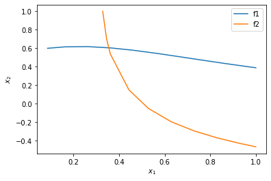
You can see now that in this range, there is only one intersection, i.e. one solution, and it is near \(x_1=0.4, x_2=0.6\). We can finally use that as an initial guess to find the only solution in this region, with confidence we are not missing any solutions.

def objective(X):
    x1, x2 = X
    return [f1(x1, x2), f2(x1, x2)]

fsolve(objective, [0.4, 0.6])
array([0.35324662, 0.60608174])

That is the same solution as reported at the Matlab site. Another use of autograd for the win here.

Copyright (C) 2019 by John Kitchin. See the License for information about copying.

org-mode source

Org-mode version = 9.2.3

Discuss on Twitter

Solving differential algebraic equations with help from autograd

| categories: dae, autograd, ode | tags:

This problem is adapted from one in "Problem Solving in Chemical Engineering with Numerical Methods, Michael B. Cutlip, Mordechai Shacham".

In the binary, batch distillation of benzene (1) and toluene (2), the moles of liquid \(L\) remaining as a function of the mole fraction of toluene (\(x_2\)) is expressed by:

\(\frac{dL}{dx_2} = \frac{L}{x_2 (k_2 - 1)}\)

where \(k_2\) is the vapor liquid equilibrium ratio for toluene. This can be computed as:

\(k_i = P_i / P\) where \(P_i = 10^{A_i + \frac{B_i}{T +C_i}}\) and that pressure is in mmHg, and the temperature is in degrees Celsius.

One difficulty in solving this problem is that the temperature is not constant; it changes with the composition. We know that the temperature changes to satisfy this constraint \(k_1(T) x_1 + k_2(T) x_2 = 1\).

Sometimes, one can solve for T directly, and substitute it into the first ODE, but this is not a possibility here. One way you might solve this is to use the constraint to find \(T\) inside an ODE function, but that is tricky; nonlinear algebra solvers need a guess and don't always converge, or may converge to non-physical solutions. They also require iterative solutions, so they will be slower than an approach where we just have to integrate the solution. A better way is to derive a second ODE \(dT/dx_2\) from the constraint. The constraint is implicit in \(T\), so We compute it as \(dT/dx_2 = -df/dx_2 / df/dT\) where \(f(x_2, T) = k_1(T) x_1 + k_2(T) x_2 - 1 = 0\). This equation is used to compute the bubble point temperature. Note, it is possible to derive these analytically, but who wants to? We can use autograd to get those derivatives for us instead.

The following information is given:

The total pressure is fixed at 1.2 atm, and the distillation starts at \(x_2=0.4\). There are initially 100 moles in the distillation.

species A B C
benzene 6.90565 -1211.033 220.79
toluene 6.95464 -1344.8 219.482

We have to start by finding the initial temperature from the constraint.

import autograd.numpy as np
from autograd import grad
from scipy.integrate import solve_ivp
from scipy.optimize import fsolve
%matplotlib inline
import matplotlib.pyplot as plt

P = 760 * 1.2 # mmHg
A1, B1, C1 = 6.90565, -1211.033,  220.79
A2, B2, C2 = 6.95464, -1344.8, 219.482

def k1(T):
    return 10**(A1 + B1 / (C1 + T)) / P

def k2(T):
    return 10**(A2 + B2 / (C2 + T)) / P

def f(x2, T):
    x1 = 1 - x2
    return k1(T) * x1 + k2(T) * x2 - 1

T0, = fsolve(lambda T: f(0.4, T), 96)
print(f'The initial temperature is {T0:1.2f} degC.')

The initial temperature is 95.59 degC.

Next, we compute the derivative we need. This derivative is derived from the constraint, which should ensure that the temperature changes as required to maintain the constraint.

dfdx2 = grad(f, 0)
dfdT = grad(f, 1)

def dTdx2(x2, T):
    return -dfdx2(x2, T) / dfdT(x2, T)

def ode(x2, X):
    L, T = X
    dLdx2 = L / (x2 * (k2(T) - 1))
    return [dLdx2, dTdx2(x2, T)]

Next we solve and plot the ODE.

x2span = (0.4, 0.8)
X0 = (100, T0)
sol = solve_ivp(ode, x2span, X0, max_step=0.01)

plt.plot(sol.t, sol.y.T)
plt.legend(['L', 'T']);
plt.xlabel('$x_2$')
plt.ylabel('L, T')
x2 = sol.t
L, T = sol.y
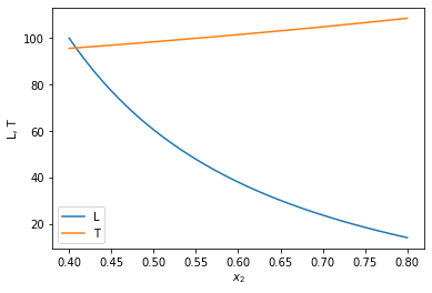
print(f'At x2={x2[-1]:1.2f} there are {L[-1]:1.2f} moles of liquid left at {T[-1]:1.2f} degC')

At x2=0.80 there are 14.04 moles of liquid left at 108.57 degC

<Figure size 432x288 with 1 Axes>

You can see that the liquid level drops, and the temperature rises.

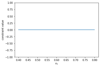
Let's double check that the constraint is actually met. We do that qualitatively here by plotting it, and quantitatively by showing all values are close to 0.

constraint = k1(T) * (1 - x2) + k2(T) * x2 - 1
plt.plot(x2, constraint)
plt.ylim([-1, 1])
plt.xlabel('$x_2$')
plt.ylabel('constraint value')
print(np.allclose(constraint, np.zeros_like(constraint)))
constraint

True

array([ 2.22044605e-16,  4.44089210e-16,  2.22044605e-16,  0.00000000e+00,
        1.11022302e-15,  0.00000000e+00,  6.66133815e-16,  0.00000000e+00,
       -2.22044605e-16,  1.33226763e-15,  8.88178420e-16, -4.44089210e-16,
        4.44089210e-16,  1.11022302e-15, -2.22044605e-16,  0.00000000e+00,
       -2.22044605e-16, -1.11022302e-15,  4.44089210e-16,  0.00000000e+00,
       -4.44089210e-16,  4.44089210e-16, -6.66133815e-16, -4.44089210e-16,
        4.44089210e-16, -1.11022302e-16, -8.88178420e-16, -8.88178420e-16,
       -9.99200722e-16, -3.33066907e-16, -7.77156117e-16, -2.22044605e-16,
       -9.99200722e-16, -1.11022302e-15, -3.33066907e-16, -1.99840144e-15,
       -1.33226763e-15, -2.44249065e-15, -1.55431223e-15, -6.66133815e-16,
       -2.22044605e-16])
<Figure size 432x288 with 1 Axes>

So indeed, the constraint is met! Once again, autograd comes to the rescue in making a computable derivative from an algebraic constraint so that we can solve a DAE as a set of ODEs using our regular machinery. Nice work autograd!

Copyright (C) 2019 by John Kitchin. See the License for information about copying.

org-mode source

Org-mode version = 9.2.3

Discuss on Twitter
« Previous Page -- Next Page »