The Kitchin Research Group

For simplicity, I am going to approximate the integral with the trapezoid method in vectorized form. Here is our program to define \(\phi(\alpha)\). I found we need a pretty dense grid on the x value so that we have a pretty accurate integral, especially near \(x=0\) where there is a singularity as α goes to zero. That doesn't worry me too much, there are better integral approximations to use, including Simpson's method, adaptive methods and perhaps quadrature. If you define them so autograd can use them, they should all work. I chose the trapezoidal method because it is simple to implement here. Note, however, the autograd.numpy wrappers don't have a definition for numpy.trapz to use it directly. You could add one, or just do this.

import autograd.numpy as np
from autograd import grad

def trapz(y, x):
    d = np.diff(x)
    return np.sum((y[0:-1] + y[1:]) * d / 2)


def phi(alpha):
    x = np.linspace(0, 1, 1000)
    y = alpha / (x**2 + alpha**2)
    return trapz(y, x)


# This is the derivative here!
adphi = grad(phi, 0)

Now, we can plot the derivatives. I will plot both the analytical and automatic differentiated results.

%matplotlib inline
import matplotlib.pyplot as plt

# results from AD
alpha = np.linspace(0.01, 1)

# The AD derivative function is not vectorized, so we use this list comprehension.
dphidalpha = [adphi(a) for a in alpha]

def analytical_dphi(alpha):
    return -1 / (1 + alpha**2)

plt.plot(alpha, analytical_dphi(alpha), label='analytical')
plt.plot(alpha, dphidalpha, 'r--', label='AD')
plt.xlabel(r'$\alpha$')
plt.ylabel(r'$frac{d\phi}{d\alpha}$')
plt.legend()

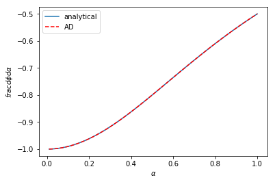
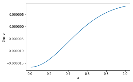
Visually, these are indistinguishable from each other. We can look at the errors too, and here we see they are negligible, and probably we can attribute them to the approximation we use for the integral, and not due to automatic differentiation.

perr = (analytical_dphi(alpha) - dphidalpha) / analytical_dphi(alpha) * 100
plt.plot(alpha, perr, label='analytical')
plt.xlabel(r'$\alpha$')
plt.ylabel('%error')

In example 2 there is this function, which has variable limits:

\(f(x) = \int_{\sin x}^{\cos x} \cosh t^2 dt\)

What is \(f'(x)\) here? It can be derived with some effort and it is:

\(f'(x) = -\cosh(\cos^2 x) \sin x - \cosh(\sin^2 x) \cos x\)

This function was kind of fun to code up, I hadn't thought about how to represent variable limits, but here it is.

def f(x):
    a = np.sin(x)
    b = np.cos(x)
    t = np.linspace(a, b, 1000)
    y = np.cosh(t**2)
    return trapz(y, t)

# Here is our derivative!
dfdx = grad(f, 0)

Here is a graphical comparison of the two:

x = np.linspace(0, 2 * np.pi)

analytical = -np.cosh(np.cos(x)**2) * np.sin(x) - \
    np.cosh(np.sin(x)**2) * np.cos(x)
ad = [dfdx(_x) for _x in x]

plt.plot(x, analytical, label='analytical')
plt.plot(x, ad, 'r--', label='AD')
plt.xlabel('x')
plt.ylabel('df/dx')
plt.legend()

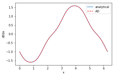
These are once again indistinguishable.

These are amazing results to me. Before trying it, I would not have thought it would be so easy to evaluate the derivative of these functions. These work of course because all the operations involved in computing the integral are differentiable and defined in autograd. It certainly opens the door to all kinds of new approaches to solving engineering problems that need the derivatives for various purposes like optimization, sensitivity analysis, etc.