The Kitchin Research Group

Last time I wrote about using automatic differentiation to find the derivative of an integral function. A related topic is finding derivatives of functions that are defined by differential equations. We typically use a numerical integrator to find solutions to these functions. Those leave us with numeric solutions which we then have to use to approximate derivatives. What if the integrator itself was differentiable? It is after all, just a program, and automatic differentiation should be able to tell us the derivatives of functions that use them. This is not a new idea, there is already a differentiable ODE solver in Tensorflow. Here I will implement a simple Runge Kutta integrator and then show how we can use automatic differentiation to do sensitivity analysis on the numeric solution.

I previously used autograd for sensitivity analysis on analytical solutions in this post. Here I will compare those results to the results from sensitivity analysis on the numerical solutions.

First, we need an autograd compatible ODE integrator. Here is one implementation of a simple, fourth order Runge-Kutta integrator. Usually, I would use indexing to do this, but that was not compatible with autograd, so I just accumulate the solution. This is a limitation of autograd, and it is probably not an issue with Tensorflow, for example, or probably pytorch. Those are more sophisticated, and more difficult to use packages than autograd. Here I am just prototyping an idea, so we stick with autograd.

import autograd.numpy as np
from autograd import grad
%matplotlib inline
import matplotlib.pyplot as plt

def rk4(f, tspan, y0, N=50):
    x, h = np.linspace(*tspan, N, retstep=True)
    y = []
    y = y + [y0]
    for i in range(0, len(x) - 1):
        k1 = h * f(x[i], y[i])
        k2 = h * f(x[i] + h / 2, y[i] + k1 / 2)
        k3 = h * f(x[i] + h / 2, y[i] + k2 / 2)
        k4 = h * f(x[i + 1], y[i] + k3)
        y += [y[-1] + (k1 + (2 * k2) + (2 * k3) + k4) / 6]
    return x, y

Now, we just check that it works as expected:

Ca0 = 1.0
k1 = k_1 = 3.0

def dCdt(t, Ca):
    return -k1 * Ca + k_1 * (Ca0 - Ca)

t, Ca = rk4(dCdt, (0, 0.5), Ca0)

def analytical_A(t, k1, k_1):
    return Ca0 / (k1 + k_1) * (k1 * np.exp(-(k1 + k_1) * t) + k_1)

plt.plot(t, Ca, label='RK4')
plt.plot(t, analytical_A(t, k1, k_1), 'r--', label='analytical')
plt.xlabel('t')
plt.ylabel('[A]')
plt.xlim([0, 0.5])
plt.ylim([0.5, 1])
plt.legend()

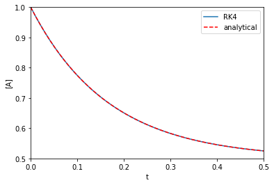
That looks fine, we cannot visually distinguish the two solutions, and they both look like Figure 1 in this paper. Note the analytical solution is not that complex, but it would not take much variation of the rate law to make this solution difficult to derive.

Next, to do sensitivity analysis, we need to define a function for \(A\) that depends on the rate constants, so we can take a derivative of it with respect to the parameters we want the sensitivity from. We seek the derivatives: \(\frac{dC_A}{dk_1}\) and \(\frac{dC_A}{dk_{-1}}\). Here is a function that does that. It will return the value of [A] at \(t\) given an initial concentration and the rate constants.

def A(Ca0, k1, k_1, t):
    def dCdt(t, Ca):
        return -k1 * Ca + k_1 * (Ca0 - Ca)
    t, Ca_ = rk4(dCdt, (0, t), Ca0)
    return Ca_[-1]

# Here are the two derivatives we seek.
dCadk1 = grad(A, 1)
dCadk_1 = grad(A, 2)

We also use autograd to get the derivatives from the analytical solution for comparison.

dAdk1 = grad(analytical_A, 1)
dAdk_1 = grad(analytical_A, 2)

Now, we can plot the sensitivities over the time range and compare them. I use the list comprehensions here because the AD functions aren't vectorized.

tspan = np.linspace(0, 0.5)

# From the numerical solutions
k1_sensitivity = [dCadk1(1.0, 3.0, 3.0, t) for t in tspan]
k_1_sensitivity = [dCadk_1(1.0, 3.0, 3.0, t) for t in tspan]

# from the analytical solutions
ak1_sensitivity = [dAdk1(t, 3.0, 3.0) for t in tspan]
ak_1_sensitivity = [dAdk_1(t, 3.0, 3.0) for t in tspan]

plt.plot(tspan, np.abs(ak1_sensitivity), 'b-', label='k1 analytical')
plt.plot(tspan, np.abs(k1_sensitivity), 'y--', label='k1 numerical')

plt.plot(tspan, np.abs(ak_1_sensitivity), 'r-', label='k_1 analytical')
plt.plot(tspan, np.abs(k_1_sensitivity), 'k--', label='k_1 numerical')

plt.xlim([0, 0.5])
plt.ylim([0, 0.1])
plt.legend()
plt.xlabel('t')
plt.ylabel('sensitivity')

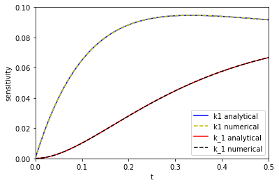
The two approaches are indistinguishable on paper. I will note that it takes a lot longer to make the graph from the numerical solution than from the analytical solution because at each point you have to reintegrate the solution from the beginning, which is certainly not efficient. That is an implementation detail that could probably be solved, at the expense of making the code look different than the way I would normally think about the problem.

On the other hand, it is remarkable we get derivatives from the numerical solution, and they look really good! That means we could do sensitivity analysis on more complex reactions, and still have a reasonable way to get sensitivity. The work here is a long way from that. My simple Runge-Kutta integrator isn't directly useful for systems of ODEs, it wouldn't work well on stiff problems, the step size isn't adaptive, etc. The Tensorflow implementation might be more suitable for this though, and maybe this post is motivation to learn how to use it!

Copyright (C) 2018 by John Kitchin. See the License for information about copying.

org-mode source

Org-mode version = 9.1.13

This paper describes how sensitivity analysis requires access to the derivatives of a function. Say, for example we have a function describing the time evolution of the concentration of species A:

\([A] = \frac{[A]_0}{k_1 + k_{-1}} (k_1 e^{(-(k_1 _ k_{-1})t)} + k_{-1})\)

The local sensitivity of the concentration of A to the parameters \(k1\) and \(k_1\) are defined as \(\frac{\partial A}{\partial k1}\) and \(\frac{\partial A}{\partial k_1}\). Our goal is to plot the sensitivity as a function of time. We could derive those derivatives, but we will use auto-differentiation instead through the autograd package. Here we import numpy from the autograd package and plot the function above.

import autograd.numpy as np

A0 = 1.0

def A(t, k1, k_1):
    return A0 / (k1 + k_1) * (k1 * np.exp(-(k1 + k_1) * t) + k_1)

%matplotlib inline
import matplotlib.pyplot as plt

t = np.linspace(0, 0.5)

k1 = 3.0
k_1 = 3.0
plt.plot(t, A(t, k1, k_1))
plt.xlim([0, 0.5])
plt.ylim([0, 1])
plt.xlabel('t')
plt.ylabel('A')

The figure above reproduces Fig. 1 from the paper referenced above. Next, we use autograd to get the derivatives. This is subtly different than our previous post. First, we need the derivative of the function with respect to the second and third arguments; the default is the first argument. Second, we want to evaluate this derivative at each time value. We use the jacobian function in autograd to get these. This is different than grad, which will sum up the derivatives at each time. That might be useful for regression, but not for sensitivity analysis. Finally, to reproduce Figure 2a, we plot the absolute value of the sensitivities.

from autograd import jacobian

dAdk1 = jacobian(A, 1)
dAdk_1 = jacobian(A, 2)

plt.plot(t, np.abs(dAdk1(t, k1, k_1)))
plt.plot(t, np.abs(dAdk_1(t, k1, k_1)))
plt.xlim([0, 0.5])
plt.ylim([0, 0.1])
plt.xlabel('t')
plt.legend(['$S_{k1}$', '$S_{k\_1}$'])

That looks like the figure in the paper. To summarize the main takeaway, autograd enabled us to readily compute derivatives without having to derive them manually. There was a little subtlety in choosing jacobian over grad or elementwise_grad but once you know what these do, it seems reasonable. It is important to import the wrapped numpy first, to enable autograd to do its work. All the functions here are pretty standard, so everything worked out of the box. We should probably be using autograd, or something like it for more things in science!

Copyright (C) 2017 by John Kitchin. See the License for information about copying.

org-mode source

Org-mode version = 9.1.2