Lather, rinse and repeat

| categories: recursive, math | tags:

Matlab post

Recursive functions are functions that call themselves repeatedly until some exit condition is met. Today we look at a classic example of recursive function for computing a factorial. The factorial of a non-negative integer n is denoted n!, and is defined as the product of all positive integers less than or equal to n.

The key ideas in defining a recursive function is that there needs to be some logic to identify when to terminate the function. Then, you need logic that calls the function again, but with a smaller part of the problem. Here we recursively call the function with n-1 until it gets called with n=0. 0! is defined to be 1.

def recursive_factorial(n):
    '''compute the factorial recursively. Note if you put a negative
    number in, this function will never end. We also do not check if
    n is an integer.'''
    if n == 0:
        return 1
    else:
        return n * recursive_factorial(n - 1)

print recursive_factorial(5)
120
from scipy.misc import factorial
print factorial(5)
120.0

0.1 Compare to a loop solution

This example can also be solved by a loop. This loop is easier to read and understand than the recursive function. Note the recursive nature of defining the variable as itself times a number.

n = 5
factorial_loop = 1
for i in range(1, n + 1):
    factorial_loop *= i

print factorial_loop
120

There are some significant differences in this example than in Matlab.

  1. the syntax of the for loop is quite different with the use of the in operator.
  2. python has the nice *= operator to replace a = a * i
  3. We have to loop from 1 to n+1 because the last number in the range is not returned.

1 Conclusions

Recursive functions have a special niche in mathematical programming. There is often another way to accomplish the same goal. That is not always true though, and in a future post we will examine cases where recursion is the only way to solve a problem.

Copyright (C) 2013 by John Kitchin. See the License for information about copying.
org-mode source

Discuss on Twitter

Integrating functions in python

| categories: math, python | tags:

Matlab post

Problem statement

find the integral of a function f(x) from a to b i.e.

$$\int_a^b f(x) dx$$

In python we use numerical quadrature to achieve this with the scipy.integrate.quad command.

as a specific example, lets integrate

$$y=x^2$$

from x=0 to x=1. You should be able to work out that the answer is 1/3.

from scipy.integrate import quad

def integrand(x):
    return x**2

ans, err = quad(integrand, 0, 1)
print ans
0.333333333333

1 double integrals

we use the scipy.integrate.dblquad command

Integrate \(f(x,y)=y sin(x)+x cos(y)\) over

\(\pi <= x <= 2\pi\)

\(0 <= y <= \pi\)

i.e.

\(\int_{x=\pi}^{2\pi}\int_{y=0}^{\pi}y sin(x)+x cos(y)dydx\)

The syntax in dblquad is a bit more complicated than in Matlab. We have to provide callable functions for the range of the y-variable. Here they are constants, so we create lambda functions that return the constants. Also, note that the order of arguments in the integrand is different than in Matlab.

from scipy.integrate import dblquad
import numpy as np

def integrand(y, x):
    'y must be the first argument, and x the second.'
    return y * np.sin(x) + x * np.cos(y)

ans, err = dblquad(integrand, np.pi, 2*np.pi,
                   lambda x: 0,
                   lambda x: np.pi)
print ans
-9.86960440109

we use the tplquad command to integrate \(f(x,y,z)=y sin(x)+z cos(x)\) over the region

\(0 <= x <= \pi\)

\(0 <= y <= 1\)

\(-1 <= z <= 1\)

from scipy.integrate import tplquad
import numpy as np

def integrand(z, y, x):
    return y * np.sin(x) + z * np.cos(x)

ans, err = tplquad(integrand,
                   0, np.pi,  # x limits
                   lambda x: 0,
                   lambda x: 1, # y limits
                   lambda x,y: -1,
                   lambda x,y: 1) # z limits

print ans
2.0

2 Summary

scipy.integrate offers the same basic functionality as Matlab does. The syntax differs significantly for these simple examples, but the use of functions for the limits enables freedom to integrate over non-constant limits.

Copyright (C) 2013 by John Kitchin. See the License for information about copying.
org-mode source

Discuss on Twitter

Better interpolate than never

| categories: interpolation | tags:

Matlab post

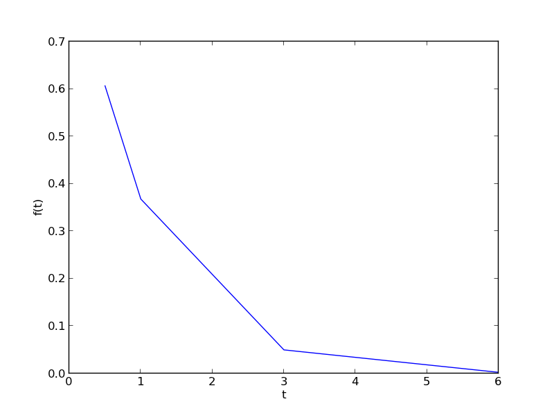
We often have some data that we have obtained in the lab, and we want to solve some problem using the data. For example, suppose we have this data that describes the value of f at time t.

import matplotlib.pyplot as plt

t = [0.5, 1, 3, 6]
f = [0.6065,    0.3679,    0.0498,    0.0025]
plt.plot(t,f)
plt.xlabel('t')
plt.ylabel('f(t)')
plt.savefig('images/interpolate-1.png')
>>> >>> >>> [<matplotlib.lines.Line2D object at 0x04D18730>]
<matplotlib.text.Text object at 0x04BEE8B0>
<matplotlib.text.Text object at 0x04C03970>

1 Estimate the value of f at t=2.

This is a simple interpolation problem.

from scipy.interpolate import interp1d

g = interp1d(t, f) # default is linear interpolation

print g(2)
print g([2, 3, 4])
>>> >>> >>> 0.20885
[ 0.20885     0.0498      0.03403333]

The function we sample above is actually f(t) = exp(-t). The linearly interpolated example is not too accurate.

import numpy as np
print np.exp(-2)
0.135335283237

2 improved interpolation?

we can tell interp1d to use a different interpolation scheme such as cubic polynomial splines like this. For nonlinear functions, this may improve the accuracy of the interpolation, as it implicitly includes information about the curvature by fitting a cubic polynomial over neighboring points.

g2 = interp1d(t, f, 'cubic')
print g2(2)
print g2([2, 3, 4])
0.108481818182
[ 0.10848182  0.0498      0.08428727]

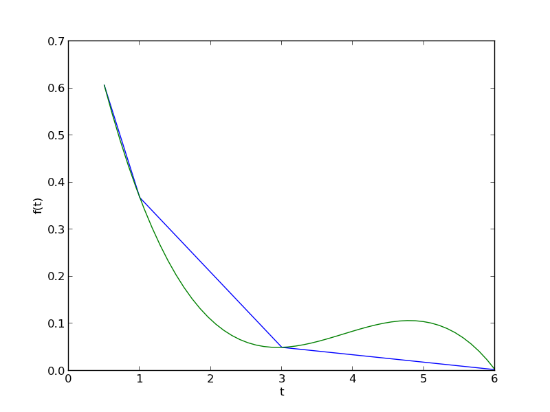
Interestingly, this is a different value than Matlab's cubic interpolation. Let us show the cubic spline fit.

plt.figure()
plt.plot(t,f)
plt.xlabel('t')
plt.ylabel('f(t)')

x = np.linspace(0.5, 6)
fit = g2(x)
plt.plot(x, fit, label='fit')
plt.savefig('images/interpolation-2.png')
<matplotlib.figure.Figure object at 0x04EF2430>
[<matplotlib.lines.Line2D object at 0x04F20ED0>]
<matplotlib.text.Text object at 0x04EF2FF0>
<matplotlib.text.Text object at 0x04F060D0>
>>> >>> >>> [<matplotlib.lines.Line2D object at 0x04F17570>]

Wow. That is a weird looking fit. Very different from what Matlab produces. This is a good teaching moment not to rely blindly on interpolation! We will rely on the linear interpolation from here out which behaves predictably.

3 The inverse question

It is easy to interpolate a new value of f given a value of t. What if we want to know the time that f=0.2? We can approach this a few ways.

3.1 method 1

We setup a function that we can use fsolve on. The function will be equal to zero at the time. The second function will look like 0 = 0.2 - f(t). The answer for 0.2=exp(-t) is t = 1.6094. Since we use interpolation here, we will get an approximate answer.

from scipy.optimize import fsolve

def func(t):
    return 0.2 - g(t)

initial_guess = 2
ans, = fsolve(func, initial_guess)
print ans
>>> ... ... >>> >>> >>> 2.0556428796

3.2 method 2: switch the interpolation order

We can switch the order of the interpolation to solve this problem. An issue we have to address in this method is that the “x” values must be monotonically increasing. It is somewhat subtle to reverse a list in python. I will use the cryptic syntax of [::-1] instead of the list.reverse() function or reversed() function. list.reverse() actually reverses the list “in place”, which changes the contents of the variable. That is not what I want. reversed() returns an iterator which is also not what I want. [::-1] is a fancy indexing trick that returns a reversed list.

g3 = interp1d(f[::-1], t[::-1])

print g3(0.2)
>>> 2.0556428796

4 A harder problem

Suppose we want to know at what time is 1/f = 100? Now we have to decide what do we interpolate: f(t) or 1/f(t). Let us look at both ways and decide what is best. The answer to \(1/exp(-t) = 100\) is 4.6052

4.1 interpolate on f(t) then invert the interpolated number

def func(t):
    'objective function. we do some error bounds because we cannot interpolate out of the range.'
    if t < 0.5: t=0.5
    if t > 6: t = 6
    return 100 - 1.0 / g(t)   

initial_guess = 4.5
a1, = fsolve(func, initial_guess)
print a1
print 'The %error is {0:%}'.format((a1 - 4.6052)/4.6052)
... ... ... ... >>> >>> >>> 5.52431289641
The %error is 19.958154%

4.2 invert f(t) then interpolate on 1/f

ig = interp1d(t, 1.0 / np.array(f))

def ifunc(t):
    if t < 0.5: t=0.5
    if t > 6: t = 6
    return 100 - ig(t)   

initial_guess = 4.5
a2, = fsolve(ifunc, initial_guess)
print a2
print 'The %error is {0:%}'.format((a2 - 4.6052)/4.6052)
>>> ... ... ... ... >>> >>> >>> 3.6310782241
The %error is -21.152649%

5 Discussion

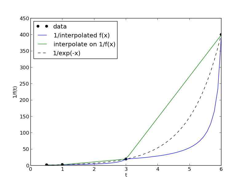
In this case you get different errors, one overestimates and one underestimates the answer, and by a lot: ± 20%. Let us look at what is happening.

import matplotlib.pyplot as plt
import numpy as np
from scipy.interpolate import interp1d

t = [0.5, 1, 3, 6]
f = [0.6065,    0.3679,    0.0498,    0.0025]

x = np.linspace(0.5, 6)


g = interp1d(t, f) # default is linear interpolation
ig = interp1d(t, 1.0 / np.array(f))

plt.figure()
plt.plot(t, 1 / np.array(f), 'ko ', label='data')
plt.plot(x, 1 / g(x), label='1/interpolated f(x)')
plt.plot(x, ig(x), label='interpolate on 1/f(x)')
plt.plot(x, 1 / np.exp(-x), 'k--', label='1/exp(-x)')
plt.xlabel('t')
plt.ylabel('1/f(t)')
plt.legend(loc='best')
plt.savefig('images/interpolation-3.png')

You can see that the 1/interpolated f(x) underestimates the value, while interpolated (1/f(x)) overestimates the value. This is an example of where you clearly need more data in that range to make good estimates. Neither interpolation method is doing a great job. The trouble in reality is that you often do not know the real function to do this analysis. Here you can say the time is probably between 3.6 and 5.5 where 1/f(t) = 100, but you can not read much more than that into it. If you need a more precise answer, you need better data, or you need to use an approach other than interpolation. For example, you could fit an exponential function to the data and use that to estimate values at other times.

So which is the best to interpolate? I think you should interpolate the quantity that is linear in the problem you want to solve, so in this case I think interpolating 1/f(x) is better. When you use an interpolated function in a nonlinear function, strange, unintuitive things can happen. That is why the blue curve looks odd. Between data points are linear segments in the original interpolation, but when you invert them, you cause the curvature to form.

Copyright (C) 2013 by John Kitchin. See the License for information about copying.
org-mode source

Discuss on Twitter

Solving a second order ode

| categories: math, ode | tags:

Matlab post

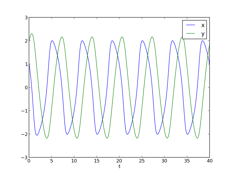
The odesolvers in scipy can only solve first order ODEs, or systems of first order ODES. To solve a second order ODE, we must convert it by changes of variables to a system of first order ODES. We consider the Van der Pol oscillator here:

$$\frac{d^2x}{dt^2} - \mu(1-x^2)\frac{dx}{dt} + x = 0$$

\(\mu\) is a constant. If we let \(y=x - x^3/3\) http://en.wikipedia.org/wiki/Van_der_Pol_oscillator, then we arrive at this set of equations:

$$\frac{dx}{dt} = \mu(x-1/3x^3-y)$$

$$\frac{dy}{dt} = \mu/x$$

here is how we solve this set of equations. Let \(\mu=1\).

from scipy.integrate import odeint
import numpy as np

mu = 1.0

def vanderpol(X, t):
    x = X[0]
    y = X[1]
    dxdt = mu * (x - 1./3.*x**3 - y)
    dydt = x / mu
    return [dxdt, dydt]

X0 = [1, 2]
t = np.linspace(0, 40, 250)

sol = odeint(vanderpol, X0, t)

import matplotlib.pyplot as plt
x = sol[:, 0]
y = sol[:, 1]

plt.plot(t,x, t, y)
plt.xlabel('t')
plt.legend(('x', 'y'))
plt.savefig('images/vanderpol-1.png')

# phase portrait
plt.figure()
plt.plot(x,y)
plt.plot(x[0], y[0], 'ro')
plt.xlabel('x')
plt.ylabel('y')
plt.savefig('images/vanderpol-2.png')

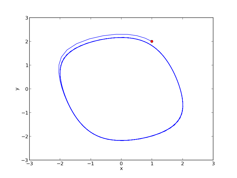
Here is the phase portrait. You can see that a limit cycle is approached, indicating periodicity in the solution.

Copyright (C) 2013 by John Kitchin. See the License for information about copying.
org-mode source

Discuss on Twitter

On the quad or trapz'd in ChemE heaven

| categories: integration, python | tags:

Matlab post

What is the difference between quad and trapz? The short answer is that quad integrates functions (via a function handle) using numerical quadrature, and trapz performs integration of arrays of data using the trapezoid method.

Let us look at some examples. We consider the example of computing \(\int_0^2 x^3 dx\). the analytical integral is \(1/4 x^4\), so we know the integral evaluates to 16/4 = 4. This will be our benchmark for comparison to the numerical methods.

We use the scipy.integrate.quad command to evaluate this \(\int_0^2 x^3 dx\).

from scipy.integrate import quad

ans, err = quad(lambda x: x**3, 0, 2)
print ans
4.0

you can also define a function for the integrand.

from scipy.integrate import quad

def integrand(x):
    return x**3

ans, err = quad(integrand, 0, 2)
print ans
4.0

1 Numerical data integration

if we had numerical data like this, we use trapz to integrate it

import numpy as np

x = np.array([0, 0.5, 1, 1.5, 2])
y = x**3

i2 = np.trapz(y, x)

error = (i2 - 4)/4

print i2, error
4.25 0.0625

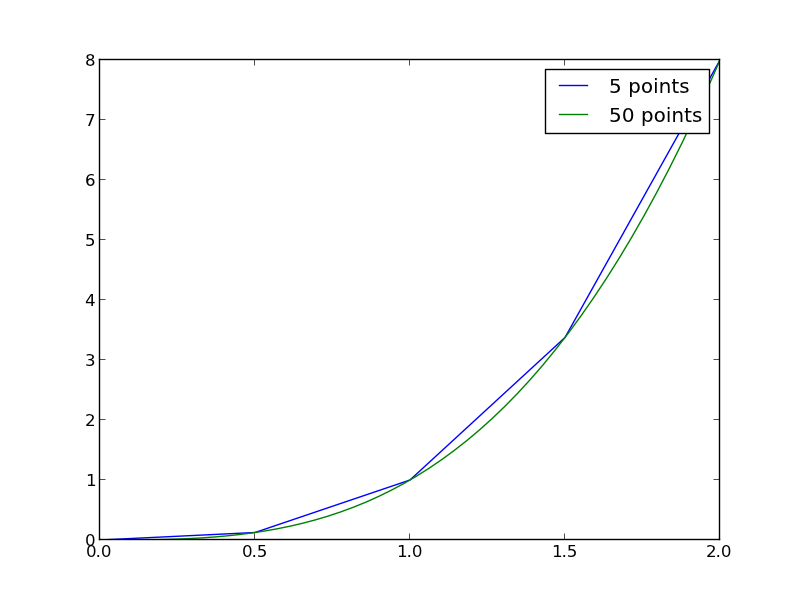
Note the integral of these vectors is greater than 4! You can see why here.

import numpy as np
import matplotlib.pyplot as plt
x = np.array([0, 0.5, 1, 1.5, 2])
y = x**3

x2 = np.linspace(0, 2)
y2 = x2**3

plt.plot(x, y, label='5 points')
plt.plot(x2, y2, label='50 points')
plt.legend()
plt.savefig('images/quad-1.png')

The trapezoid method is overestimating the area significantly. With more points, we get much closer to the analytical value.

import numpy as np

x2 = np.linspace(0, 2, 100)
y2 = x2**3

print np.trapz(y2, x2)
4.00040812162

2 Combining numerical data with quad

You might want to combine numerical data with the quad function if you want to perform integrals easily. Let us say you are given this data:

x = [0 0.5 1 1.5 2]; y = [0 0.1250 1.0000 3.3750 8.0000];

and you want to integrate this from x = 0.25 to 1.75. We do not have data in those regions, so some interpolation is going to be needed. Here is one approach.

from scipy.interpolate import interp1d
from scipy.integrate import quad
import numpy as np

x = [0, 0.5, 1, 1.5, 2]
y = [0,    0.1250,    1.0000,    3.3750,    8.0000]

f = interp1d(x, y)

# numerical trapezoid method
xfine = np.linspace(0.25, 1.75)
yfine = f(xfine)
print np.trapz(yfine, xfine)

# quadrature with interpolation
ans, err = quad(f, 0.25, 1.75)
print ans
2.53199187838
2.53125

These approaches are very similar, and both rely on linear interpolation. The second approach is simpler, and uses fewer lines of code.

3 Summary

trapz and quad are functions for getting integrals. Both can be used with numerical data if interpolation is used. The syntax for the quad and trapz function is different in scipy than in Matlab.

Finally, see this post for an example of solving an integral equation using quad and fsolve.

Copyright (C) 2013 by John Kitchin. See the License for information about copying.
org-mode source

Discuss on Twitter
« Previous Page -- Next Page »