Constrained minimization to find equilibrium compositions

| categories: optimization | tags: thermodynamics, reaction engineering

adapated from Chemical Reactor analysis and design fundamentals, Rawlings and Ekerdt, appendix A.2.3.

Matlab post

The equilibrium composition of a reaction is the one that minimizes the total Gibbs free energy. The Gibbs free energy of a reacting ideal gas mixture depends on the mole fractions of each species, which are determined by the initial mole fractions of each species, the extent of reactions that convert each species, and the equilibrium constants.

Reaction 1: \(I + B \rightleftharpoons P1\)

Reaction 2: \(I + B \rightleftharpoons P2\)

Here we define the Gibbs free energy of the mixture as a function of the reaction extents.

import numpy as np

def gibbs(E):
    'function defining Gibbs free energy as a function of reaction extents'
    e1 = E[0]
    e2 = E[1]
    # known equilibrium constants and initial amounts
    K1 = 108; K2 = 284; P = 2.5
    yI0 = 0.5; yB0 = 0.5; yP10 = 0.0; yP20 = 0.0
    # compute mole fractions
    d = 1 - e1 - e2
    yI = (yI0 - e1 - e2) / d
    yB = (yB0 - e1 - e2) / d
    yP1 = (yP10 + e1) / d
    yP2 = (yP20 + e2) / d
    G = (-(e1 * np.log(K1) + e2 * np.log(K2)) +
         d * np.log(P) + yI * d * np.log(yI) +
         yB * d * np.log(yB) + yP1 * d * np.log(yP1) + yP2 * d * np.log(yP2))
    return G

The equilibrium constants for these reactions are known, and we seek to find the equilibrium reaction extents so we can determine equilibrium compositions. The equilibrium reaction extents are those that minimize the Gibbs free energy. We have the following constraints, written in standard less than or equal to form:

\(-\epsilon_1 \le 0\)

\(-\epsilon_2 \le 0\)

\(\epsilon_1 + \epsilon_2 \le 0.5\)

In Matlab we express this in matrix form as Ax=b where

\begin{equation} A = \left[ \begin{array}{cc} -1 & 0 \\ 0 & -1 \\ 1 & 1 \end{array} \right] \end{equation}

and

\begin{equation} b = \left[ \begin{array}{c} 0 \\ 0 \\ 0.5\end{array} \right] \end{equation}

Unlike in Matlab, in python we construct the inequality constraints as functions that are greater than or equal to zero when the constraint is met.

def constraint1(E):
    e1 = E[0]
    return e1


def constraint2(E):
    e2 = E[1]
    return e2


def constraint3(E):
    e1 = E[0]
    e2 = E[1]
    return 0.5 - (e1 + e2)

Now, we minimize.

from scipy.optimize import fmin_slsqp

X0 = [0.2, 0.2]
X = fmin_slsqp(gibbs, X0, ieqcons=[constraint1, constraint2, constraint3],
               bounds=((0.001, 0.499),
                       (0.001, 0.499)))
print(X)

print(gibbs(X))
Optimization terminated successfully.    (Exit mode 0)
            Current function value: -2.55942394906
            Iterations: 7
            Function evaluations: 31
            Gradient evaluations: 7
[ 0.13336503  0.35066486]
-2.55942394906

One way we can verify our solution is to plot the gibbs function and see where the minimum is, and whether there is more than one minimum. We start by making grids over the range of 0 to 0.5. Note we actually start slightly above zero because at zero there are some numerical imaginary elements of the gibbs function or it is numerically not defined since there are logs of zero there. We also set all elements where the sum of the two extents is greater than 0.5 to near zero, since those regions violate the constraints.

import numpy as np
import matplotlib.pyplot as plt

def gibbs(E):
    'function defining Gibbs free energy as a function of reaction extents'
    e1 = E[0]
    e2 = E[1]
    # known equilibrium constants and initial amounts
    K1 = 108; K2 = 284; P = 2.5;
    yI0 = 0.5; yB0 = 0.5; yP10 = 0.0; yP20 = 0.0;
    # compute mole fractions
    d = 1 - e1 - e2;
    yI = (yI0 - e1 - e2)/d;
    yB = (yB0 - e1 - e2)/d;
    yP1 = (yP10 + e1)/d;
    yP2 = (yP20 + e2)/d;
    G = (-(e1 * np.log(K1) + e2 * np.log(K2)) +
         d * np.log(P) + yI * d * np.log(yI) +
         yB * d * np.log(yB) + yP1 * d * np.log(yP1) + yP2 * d * np.log(yP2))
    return G


a = np.linspace(0.001, 0.5, 100)
E1, E2 = np.meshgrid(a,a)

sumE = E1 + E2
E1[sumE >= 0.5] = 0.00001
E2[sumE >= 0.5] = 0.00001

# now evaluate gibbs
G = np.zeros(E1.shape)
m,n = E1.shape

G = gibbs([E1, E2])

CS = plt.contour(E1, E2, G, levels=np.linspace(G.min(),G.max(),100))
plt.xlabel('$\epsilon_1$')
plt.ylabel('$\epsilon_2$')
plt.colorbar()

plt.plot([0.13336503],  [0.35066486], 'ro')

plt.savefig('images/gibbs-minimization-1.png')
plt.savefig('images/gibbs-minimization-1.svg')
plt.show()

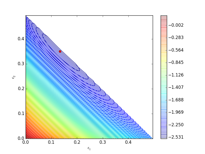
You can see we found the minimum. We can compute the mole fractions pretty easily.

e1 = X[0];
e2 = X[1];

yI0 = 0.5; yB0 = 0.5; yP10 = 0; yP20 = 0; #initial mole fractions

d = 1 - e1 - e2;
yI = (yI0 - e1 - e2) / d
yB = (yB0 - e1 - e2) / d
yP1 = (yP10 + e1) / d
yP2 = (yP20 + e2) / d

print('y_I = {0:1.3f} y_B = {1:1.3f} y_P1 = {2:1.3f} y_P2 = {3:1.3f}'.format(yI,yB,yP1,yP2))
y_I = 0.031 y_B = 0.031 y_P1 = 0.258 y_P2 = 0.680

1 summary

I found setting up the constraints in this example to be more confusing than the Matlab syntax.

Copyright (C) 2016 by John Kitchin. See the License for information about copying.

org-mode source

Org-mode version = 8.2.10

Discuss on Twitter

Time dependent concentration in a first order reversible reaction in a batch reactor

| categories: ode | tags: reaction engineering

Matlab post

Given this reaction \(A \rightleftharpoons B\), with these rate laws:

forward rate law: \(-r_a = k_1 C_A\)

backward rate law: \(-r_b = k_{-1} C_B\)

plot the concentration of A vs. time. This example illustrates a set of coupled first order ODES.

from scipy.integrate import odeint
import numpy as np

def myode(C, t):
    # ra = -k1*Ca
    # rb = -k_1*Cb
    # net rate for production of A:  ra - rb
    # net rate for production of B: -ra + rb

    k1 = 1   # 1/min;
    k_1 = 0.5   # 1/min;

    Ca = C[0]
    Cb = C[1]

    ra = -k1 * Ca
    rb = -k_1 * Cb

    dCadt =  ra - rb
    dCbdt = -ra + rb

    dCdt = [dCadt, dCbdt]
    return dCdt

tspan = np.linspace(0, 5)

init = [1, 0]  # mol/L
C = odeint(myode, init, tspan)

Ca = C[:,0]
Cb = C[:,1]

import matplotlib.pyplot as plt
plt.plot(tspan, Ca, tspan, Cb)
plt.xlabel('Time (min)')
plt.ylabel('C (mol/L)')
plt.legend(['$C_A$', '$C_B$'])
plt.savefig('images/reversible-batch.png')

That is it. The main difference between this and Matlab is the order of arguments in odeint is different, and the ode function has differently ordered arguments.

Copyright (C) 2013 by John Kitchin. See the License for information about copying.

org-mode source

Discuss on Twitter

Estimating the boiling point of water

| categories: uncategorized | tags: thermodynamics

Matlab post

I got distracted looking for Shomate parameters for ethane today, and came across this website on predicting the boiling point of water using the Shomate equations. The basic idea is to find the temperature where the Gibbs energy of water as a vapor is equal to the Gibbs energy of the liquid.

import matplotlib.pyplot as plt

Liquid water (\url{http://webbook.nist.gov/cgi/cbook.cgi?ID=C7732185&Units=SI&Mask=2#Thermo-Condensed})

# valid over 298-500

Hf_liq = -285.830   # kJ/mol
S_liq = 0.06995     # kJ/mol/K
shomateL = [-203.6060,
            1523.290,
           -3196.413,
            2474.455,
               3.855326,
            -256.5478,
            -488.7163,
            -285.8304]

Gas phase water (\url{http://webbook.nist.gov/cgi/cbook.cgi?ID=C7732185&Units=SI&Mask=1&Type=JANAFG&Table=on#JANAFG})

Interestingly, these parameters are listed as valid only above 500K. That means we have to extrapolate the values down to 298K. That is risky for polynomial models, as they can deviate substantially outside the region they were fitted to.

Hf_gas = -241.826  # kJ/mol
S_gas = 0.188835   # kJ/mol/K

shomateG = [30.09200,
             6.832514,
             6.793435,
            -2.534480,
             0.082139,
          -250.8810,
           223.3967,
          -241.8264]

Now, we wan to compute G for each phase as a function of T

import numpy as np

T = np.linspace(0, 200) + 273.15
t = T / 1000.0

sTT = np.vstack([np.log(t),
                 t,
                 (t**2) / 2.0,
                 (t**3) / 3.0,
                 -1.0 / (2*t**2),
                 0 * t,
                 t**0,
                 0 * t**0]).T / 1000.0

hTT = np.vstack([t,
                 (t**2)/2.0,
                 (t**3)/3.0,
                 (t**4)/4.0,
                 -1.0 / t,
                 1 * t**0,
                 0 * t**0,
                 -1 * t**0]).T

Gliq = Hf_liq + np.dot(hTT, shomateL) - T*(np.dot(sTT, shomateL))
Ggas = Hf_gas + np.dot(hTT, shomateG) - T*(np.dot(sTT, shomateG))
                 
from scipy.interpolate import interp1d
from scipy.optimize import fsolve

f = interp1d(T, Gliq - Ggas)
bp, = fsolve(f, 373)
print 'The boiling point is {0} K'.format(bp)
>>> >>> >>> >>> ... ... ... ... ... ... ... >>> >>> ... ... ... ... ... ... ... >>> >>> >>> >>> ... >>> >>> >>> >>> >>> The boiling point is 373.206081312 K
plt.figure(); plt.clf()
plt.plot(T-273.15, Gliq, T-273.15, Ggas)
plt.legend(['liquid water', 'steam'])

plt.xlabel('Temperature $^\circ$C')
plt.ylabel('$\Delta G$ (kJ/mol)')
plt.title('The boiling point is approximately {0:1.2f} $^\circ$C'.format(bp-273.15))
plt.savefig('images/boiling-water.png')
<matplotlib.figure.Figure object at 0x050D2E30>
[<matplotlib.lines.Line2D object at 0x051AB610>, <matplotlib.lines.Line2D object at 0x051B4C90>]
<matplotlib.legend.Legend object at 0x051B9030>
>>> <matplotlib.text.Text object at 0x0519E390>
<matplotlib.text.Text object at 0x050FB390>
<matplotlib.text.Text object at 0x050FBFB0>

1 Summary

The answer we get us 0.05 K too high, which is not bad considering we estimated it using parameters that were fitted to thermodynamic data and that had finite precision and extrapolated the steam properties below the region the parameters were stated to be valid for.

Copyright (C) 2013 by John Kitchin. See the License for information about copying.

org-mode source

Discuss on Twitter

Using Lagrange multipliers in optimization

| categories: optimization | tags:

Matlab post (adapted from http://en.wikipedia.org/wiki/Lagrange_multipliers.)

Suppose we seek to maximize the function \(f(x,y)=x+y\) subject to the constraint that \(x^2 + y^2 = 1\). The function we seek to maximize is an unbounded plane, while the constraint is a unit circle. We want the maximum value of the circle, on the plane. We plot these two functions here.

import numpy as np

x = np.linspace(-1.5, 1.5)

[X, Y] = np.meshgrid(x, x)

import matplotlib as mpl
from mpl_toolkits.mplot3d import Axes3D
import matplotlib.pyplot as plt

fig = plt.figure()
ax = fig.gca(projection='3d')

ax.plot_surface(X, Y, X + Y)

theta = np.linspace(0,2*np.pi);
R = 1.0
x1 = R * np.cos(theta)
y1 = R * np.sin(theta)

ax.plot(x1, y1, x1 + y1, 'r-')
plt.savefig('images/lagrange-1.png')

1 Construct the Lagrange multiplier augmented function

To find the maximum, we construct the following function: \(\Lambda(x,y; \lambda) = f(x,y)+\lambda g(x,y)\) where \(g(x,y) = x^2 + y^2 - 1 = 0\), which is the constraint function. Since \(g(x,y)=0\), we are not really changing the original function, provided that the constraint is met!

import numpy as np

def func(X):
    x = X[0]
    y = X[1]
    L = X[2] # this is the multiplier. lambda is a reserved keyword in python
    return x + y + L * (x**2 + y**2 - 1)

2 Finding the partial derivatives

The minima/maxima of the augmented function are located where all of the partial derivatives of the augmented function are equal to zero, i.e. \(\partial \Lambda/\partial x = 0\), \(\partial \Lambda/\partial y = 0\), and \(\partial \Lambda/\partial \lambda = 0\). the process for solving this is usually to analytically evaluate the partial derivatives, and then solve the unconstrained resulting equations, which may be nonlinear.

Rather than perform the analytical differentiation, here we develop a way to numerically approximate the partial derivatives.

def dfunc(X):
    dLambda = np.zeros(len(X))
    h = 1e-3 # this is the step size used in the finite difference.
    for i in range(len(X)):
        dX = np.zeros(len(X))
        dX[i] = h
        dLambda[i] = (func(X+dX)-func(X-dX))/(2*h);
    return dLambda

3 Now we solve for the zeros in the partial derivatives

The function we defined above (dfunc) will equal zero at a maximum or minimum. It turns out there are two solutions to this problem, but only one of them is the maximum value. Which solution you get depends on the initial guess provided to the solver. Here we have to use some judgement to identify the maximum.

from scipy.optimize import fsolve

# this is the max
X1 = fsolve(dfunc, [1, 1, 0])
print X1, func(X1)

# this is the min
X2 = fsolve(dfunc, [-1, -1, 0])
print X2, func(X2)
>>> ... >>> [ 0.70710678  0.70710678 -0.70710678] 1.41421356237
>>> ... >>> [-0.70710678 -0.70710678  0.70710678] -1.41421356237

4 Summary

Three dimensional plots in matplotlib are a little more difficult than in Matlab (where the code is almost the same as 2D plots, just different commands, e.g. plot vs plot3). In Matplotlib you have to import additional modules in the right order, and use the object oriented approach to plotting as shown here.

Copyright (C) 2013 by John Kitchin. See the License for information about copying.

org-mode source

Discuss on Twitter

Some of this, sum of that

| categories: recursive, miscellaneous | tags:

Matlab plot

Python provides a sum function to compute the sum of a list. However, the sum function does not work on every arrangement of numbers, and it certainly does not work on nested lists. We will solve this problem with recursion.

Here is a simple example.

v = [1, 2, 3, 4, 5, 6, 7, 8, 9] # a list
print sum(v)

v = (1, 2, 3, 4, 5, 6, 7, 8, 9)  # a tuple
print sum(v)
45
45

If you have data in a dictionary, sum works by default on the keys. You can give the sum function the values like this.

v = {'a':1, 'b':3, 'c':4}
print sum(v.values())
8

1 Nested lists

Suppose now we have nested lists. This kind of structured data might come up if you had grouped several things together. For example, suppose we have 5 departments, with 1, 5, 15, 7 and 17 people in them, and in each department they are divided into groups.

Department 1: 1 person Department 2: group of 2 and group of 3 Department 3: group of 4 and 11, with a subgroups of 5 and 6 making up the group of 11. Department 4: 7 people Department 5: one group of 8 and one group of 9.

We might represent the data like this nested list. Now, if we want to compute the total number of people, we need to add up each group. We cannot simply sum the list, because some elements are single numbers, and others are lists, or lists of lists. We need to recurse through each entry until we get down to a number, which we can add to the running sum.

v = [1, 
    [2, 3],
    [4, [5, 6]],
    7,
    [8,9]]

def recursive_sum(X):
    'compute sum of arbitrarily nested lists'
    s = 0 # initial value of the sum

    for i in range(len(X)):
        import types  # we use this to test if we got a number
        if isinstance(X[i], (types.IntType,
                             types.LongType,
                             types.FloatType,
                             types.ComplexType)):
            # this is the terminal step
            s += X[i]
        else:
            # we did not get a number, so we recurse
            s += recursive_sum(X[i])
    return s

print recursive_sum(v)
print recursive_sum([1,2,3,4,5,6,7,8,9]) # test on non-nested list
45
45

In Post 1970 we examined recursive functions that could be replaced by loops. Here we examine a function that can only work with recursion because the nature of the nested data structure is arbitrary. There are arbitary branches and depth in the data structure. Recursion is nice because you do not have to define that structure in advance.

Copyright (C) 2013 by John Kitchin. See the License for information about copying.

org-mode source

Discuss on Twitter
« Previous Page -- Next Page »