Using Lagrange multipliers in optimization
Posted February 03, 2013 at 09:00 AM | categories: optimization | tags:
Updated February 27, 2013 at 02:43 PM
Matlab post (adapted from http://en.wikipedia.org/wiki/Lagrange_multipliers.)
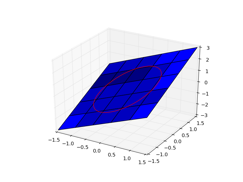
Suppose we seek to maximize the function \(f(x,y)=x+y\) subject to the constraint that \(x^2 + y^2 = 1\). The function we seek to maximize is an unbounded plane, while the constraint is a unit circle. We want the maximum value of the circle, on the plane. We plot these two functions here.
import numpy as np

x = np.linspace(-1.5, 1.5)

[X, Y] = np.meshgrid(x, x)

import matplotlib as mpl
from mpl_toolkits.mplot3d import Axes3D
import matplotlib.pyplot as plt

fig = plt.figure()
ax = fig.gca(projection='3d')

ax.plot_surface(X, Y, X + Y)

theta = np.linspace(0,2*np.pi);
R = 1.0
x1 = R * np.cos(theta)
y1 = R * np.sin(theta)

ax.plot(x1, y1, x1 + y1, 'r-')
plt.savefig('images/lagrange-1.png')
1 Construct the Lagrange multiplier augmented function
To find the maximum, we construct the following function: \(\Lambda(x,y; \lambda) = f(x,y)+\lambda g(x,y)\) where \(g(x,y) = x^2 + y^2 - 1 = 0\), which is the constraint function. Since \(g(x,y)=0\), we are not really changing the original function, provided that the constraint is met!
import numpy as np

def func(X):
    x = X[0]
    y = X[1]
    L = X[2] # this is the multiplier. lambda is a reserved keyword in python
    return x + y + L * (x**2 + y**2 - 1)
2 Finding the partial derivatives
The minima/maxima of the augmented function are located where all of the partial derivatives of the augmented function are equal to zero, i.e. \(\partial \Lambda/\partial x = 0\), \(\partial \Lambda/\partial y = 0\), and \(\partial \Lambda/\partial \lambda = 0\). the process for solving this is usually to analytically evaluate the partial derivatives, and then solve the unconstrained resulting equations, which may be nonlinear.
Rather than perform the analytical differentiation, here we develop a way to numerically approximate the partial derivatives.
def dfunc(X):
    dLambda = np.zeros(len(X))
    h = 1e-3 # this is the step size used in the finite difference.
    for i in range(len(X)):
        dX = np.zeros(len(X))
        dX[i] = h
        dLambda[i] = (func(X+dX)-func(X-dX))/(2*h);
    return dLambda
3 Now we solve for the zeros in the partial derivatives
The function we defined above (dfunc) will equal zero at a maximum or minimum. It turns out there are two solutions to this problem, but only one of them is the maximum value. Which solution you get depends on the initial guess provided to the solver. Here we have to use some judgement to identify the maximum.
from scipy.optimize import fsolve

# this is the max
X1 = fsolve(dfunc, [1, 1, 0])
print X1, func(X1)

# this is the min
X2 = fsolve(dfunc, [-1, -1, 0])
print X2, func(X2)
>>> ... >>> [ 0.70710678  0.70710678 -0.70710678] 1.41421356237
>>> ... >>> [-0.70710678 -0.70710678  0.70710678] -1.41421356237
4 Summary
Three dimensional plots in matplotlib are a little more difficult than in Matlab (where the code is almost the same as 2D plots, just different commands, e.g. plot vs plot3). In Matplotlib you have to import additional modules in the right order, and use the object oriented approach to plotting as shown here.
Copyright (C) 2013 by John Kitchin. See the License for information about copying.