A new and improved Emacs gnuplot DSL

| categories: lisp, plotting, emacs | tags:

A significant limitation of the previous DSL I wrote is that all the plotting commands have to go in one macro. It would be nice to accumulate them in different forms, and when you want to run them all. A classic way to do that in Emacs lisp is to make a global variable, e.g. *gnuplot-cmds* and append commands to it. Then when you want to, run the commands.

A more modern approach is to use a closure to encapsulate the commands. Here is a "let over lambda" that defines a few functions that encapsulate an enclosed variable gnuplot-commands. We define one function to add commands to the list of commands, one to clear the commands, one to generate the gnuplot script as a string, and one to run the program. The enclosed variable gnuplot-commands is basically only accessible by these functions. It is encapsulated, similar to if we defined a class in Python then made an instance of it with an attribute that was accessible only be instance methods. On one hand, this "protects" the variable, and keeps it out of the global namespace. On the other hand, we lose the documentation that would have come with a defvar, and we have to define a function to access the contents of that variable.

(let ((gnuplot-commands '("set terminal qt")))

  (defun gnuplot-add-cmd (s)
    "Append the command S to gnuplot-cmds."
    (setq gnuplot-commands (append gnuplot-commands (list s))))

  (defun gnuplot-clear ()
    (setq gnuplot-commands '("set terminal qt")))

  (defun gnuplot-script ()
    (s-join "\n" gnuplot-commands)))
gnuplot-script

To run the commands, we define this function. It does not need to be in the closure because it only accesses the commands through functions we defined in the closure.

(defun gnuplot-show ()
    (let* ((temporary-file-directory ".")
           (cmdfile (make-temp-file "gnuplot-cmds-" nil ".gpl"))
           (shellcmd (format "gnuplot --persist -c \"%s\"" cmdfile))
           (cmds (gnuplot-script)))
      (with-temp-file cmdfile
        (insert cmds))
      (shell-command shellcmd)
      (delete-file cmdfile)
      cmds))
gnuplot-show

Last time I noted I had a new idea for the DSL syntax that would give us more flexibility to inject variables and code into the DSL. The idea is to use keywords, symbols that start with :, to indicate they should be replaced by the value of the non-keyword symbol in the environment, and for any form that starts with : to evaluate that form. So, (: - 5 4) would get replaced by 1. Here is the new macro for that.

(defmacro kargs (&rest args)
  "Convert symbols to strings, quote strings, and (expr) to what they evaluate to."
  `(s-join " " (list ,@(cl-mapcan
                        (lambda (s)
                          (list
                           (cond
                            ((keywordp s)
                             (format "%s"
                                     (symbol-value (intern (substring (symbol-name s) 1)))))
                            ((symbolp s)
                             (symbol-name s))
                            ((stringp s)
                             (format "\"%s\"" s))
                            ((and (listp s) (eq : (car s)))
                             `(with-output-to-string
                                (princ ,(cdr s))))
                            (t
                             (format "%s" s)))))
                        args))))
kargs

Now, our gnuplot macro is simpler, since all it does is add commands to the list. If the form is a string, we add it as is, if the form starts with (: stuff) we evaluate the cdr of the form, and otherwise, we pass the form contents to the kargs macro for processing.

(defmacro gnuplot (&rest forms)
  `(loop for s in (list ,@(mapcar (lambda (x)
                                    (cond
                                     ((stringp x)
                                      x)
                                     ((and (listp x) (eq : (car x)))
                                      `,(cdr x))
                                     (t
                                      `(kargs ,@x))))
                                  forms))
         do (gnuplot-add-cmd s)))
gnuplot

What did that gain us? First, we can break up a script so we can talk about it, maybe do some calculations, etc… Let's look at the example at http://gnuplot.sourceforge.net/demo/linkedaxes.html.

We can start with the basic settings.

(gnuplot-clear)

(gnuplot
 (set terminal png)
 (set output "linkedaxes.png")
 (set encoding utf8)
 (set key outside Left)
 (set bmargin 5)
 (set tmargin 6)
 (set style data lines)
 (set tics in)
 (set ticslevel 0.5)
 (set xlabel  "X-ray energy in eV")

 (set format y  \'%5.1fe\')
 (set title " Anomalous scattering factors ")
 (set xrange  [9000:14400])
 (set offset 0\,0\,1.0\,0)
 (set xtics nomirror)
 (set link x via 12398./x inverse 12398./x)

 (set x2label  "X-ray wavelength in Å")
 (set x2tics 0.1  format "%.1f Å" nomirror))

We need to download some data files. We can do that, and add another line to the gnuplot script. The escaping on the quotes and commas is especially tedious in this one ;) but, we don't need those pesky line-continuations here.

(shell-command "wget http://skuld.bmsc.washington.edu/scatter/data/Br.dat")
(shell-command "wget http://skuld.bmsc.washington.edu/scatter/data/Ta.dat")


(gnuplot
 (plot "Br.dat" volatile using 1:3 title \'Br f\"\'  lt 1 lw 3\, \'\' volatile using 1:2 title "Br f'"  lt 1 lw 1\,
       "Ta.dat" volatile using 1:3 title \'Ta f\"\' lt 2 lw 3\, \'\' volatile using 1:2 title \"Ta f\'\"  lt 2 lw 1))

(gnuplot-script)
set terminal qt
set terminal png
set output "linkedaxes.png"
set encoding utf8
set key outside Left
set bmargin 5
set tmargin 6
set style data lines
set tics in
set ticslevel 0.5
set xlabel "X-ray energy in eV"
set format y '%5.1fe'
set title " Anomalous scattering factors "
set xrange [9000:14400]
set offset 0,0,1.0,0
set xtics nomirror
set link x via 12398./x inverse 12398./x
set x2label "X-ray wavelength in Å"
set x2tics 0.1 format "%.1f Å" nomirror
plot "Br.dat" volatile using 1:3 title 'Br f"' lt 1 lw 3, '' volatile using 1:2 title "Br f'" lt 1 lw 1, "Ta.dat" volatile using 1:3 title 'Ta f"' lt 2 lw 3, '' volatile using 1:2 title "Ta f'" lt 2 lw 1

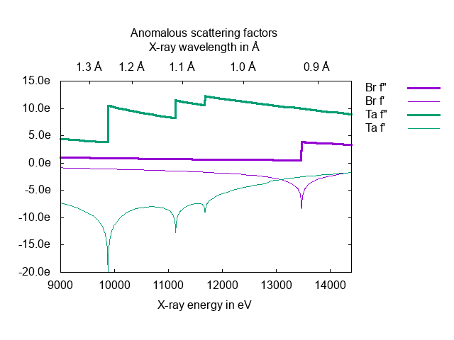
Finally, we can set the output to png, and run our program.

(gnuplot-show)

Looks good.
What about the fancy keyword formatting? Here is an example of that in action. :term gets replaced by the term variable, :png gets replaced by the filename, and :x is replaced by 4.

(gnuplot-clear)
(let ((x 4)
      (term "png")
      (png "\"polar.png\""))
  (gnuplot
   (set terminal :term)
   (set output :png)
   (set polar)
   (set dummy t)
   (plot sin\( :x *t\) \,cos\( :x *t\))
   (set offset 0\,0\,0\,0)))

(gnuplot-show)
set terminal qt
set terminal png
set output "polar.png"
set polar
set dummy t
plot sin( 4 *t) ,cos( 4 *t)
set offset 0,0,0,0
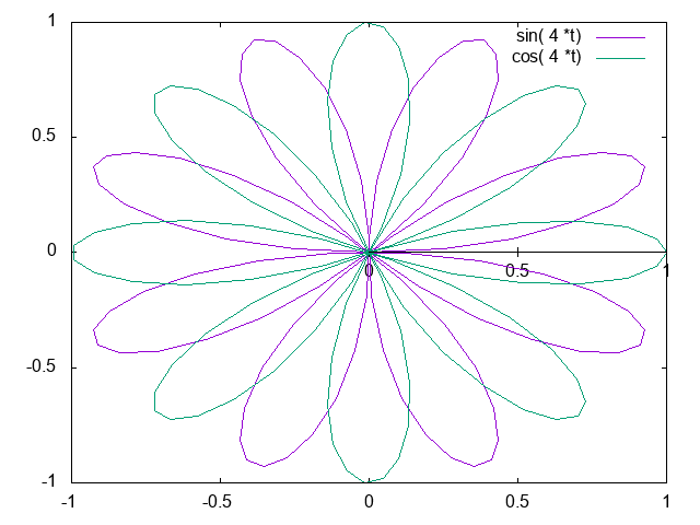
There are a few nuances I didn't expect. First, you have to escape the parentheses in this case because otherwise it looks like a form that will be ignored. Second, you have to quote the string to get quotes into the gnuplot script. Third, there has to be a space before and after the keywords for emacs to parse it correctly and do the substitution.

Let's look at one last example that uses the (: form). We reproduce a figure from http://gnuplot.sourceforge.net/demo/transparent_solids.html here.

(gnuplot-clear)
(gnuplot
 (set terminal pngcairo  background "#ffffff" enhanced font "arial,9" fontscale 1.0 size 512\, 384 )
 (set output "transparent-solids.png")
 ;; construct the title
 (set title (: format "\"%s\"" (concat "Interlocking Tori - PM3D surface" "with depth sorting and transparency")))

 ;; use lisp code to create a gnuplot command
 (: concat "unset" " " "border")

 (unset key)
 (set object 1 rect from screen 0\, 0\, 0 to screen 1\, 1\, 0 behind)
 (set object 1 rect fc  rgb \"gray\"  fillstyle solid 1.0  border -1)
 (set view 64\, 345\, 1.24375\, 0.995902)
 (set isosamples 50\, 20)
 (unset xtics)
 (unset ytics)
 (unset ztics)
 (set dummy u\,v)
 (set parametric)
 (set urange [ -pi : pi ])
 (set vrange [ -pi : pi ])

 (set style fill  transparent solid 0.30 border)
 (set pm3d depthorder)
 (set palette rgbformulae 8\, 9\, 7)
 (set pm3d interpolate 1\,1 flush begin noftriangles border lt black linewidth 0.500 dashtype solid corners2color mean)
 (set colorbox vertical origin screen 0.9\, 0.2\, 0 size screen 0.05\, 0.6\, 0 front  noinvert bdefault)

 (splot (: concat "cos(u)+.5*cos(u)*cos(v),sin(u)+.5*sin(u)*cos(v),.5*sin(v) with pm3d,"
           "1+cos(u)+.5*cos(u)*cos(v),.5*sin(v),sin(u)+.5*sin(u)*cos(v) with pm3d")))
(gnuplot-show)
set terminal qt
set terminal pngcairo background "#ffffff" enhanced font "arial,9" fontscale 1.0 size 512, 384
set output "transparent-solids.png"
set title "Interlocking Tori - PM3D surfacewith depth sorting and transparency"
unset border
unset key
set object 1 rect from screen 0, 0, 0 to screen 1, 1, 0 behind
set object 1 rect fc rgb "gray" fillstyle solid 1.0 border -1
set view 64, 345, 1.24375, 0.995902
set isosamples 50, 20
unset xtics
unset ytics
unset ztics
set dummy u,v
set parametric
set urange [-pi : pi]
set vrange [-pi : pi]
set style fill transparent solid 0.3 border
set pm3d depthorder
set palette rgbformulae 8, 9, 7
set pm3d interpolate 1,1 flush begin noftriangles border lt black linewidth 0.5 dashtype solid corners2color mean
set colorbox vertical origin screen 0.9, 0.2, 0 size screen 0.05, 0.6, 0 front noinvert bdefault
splot cos(u)+.5*cos(u)*cos(v),sin(u)+.5*sin(u)*cos(v),.5*sin(v) with pm3d,1+cos(u)+.5*cos(u)*cos(v),.5*sin(v),sin(u)+.5*sin(u)*cos(v) with pm3d
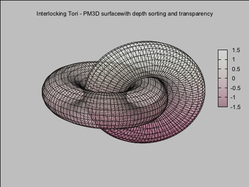
Overall this seems like an improvement to the DSL. I didn't invent the idea of reusing keywords this way out of the blue. In On Lisp, Paul graham uses "special" variable names in Chapter 18, where he shows how to use gensyms for special purposes, and also variables with special names like ?x. Even Emacs is using a variation of this idea. Check out this new let-alist macro:

(let-alist '((x . 5))
  (+ 1 .x))
6

There is a special variable inside the body that is a dot-name. The macro expands to provide a value for that symbol. I wonder if I should have tried to use an approach like this instead. Maybe another day. After I read and study the four defuns and single defmacro that make this possible!

You can see here what happens:

(macroexpand '(let-alist '((x . 5))
  (+ 1 .x)))
(let
    ((alist
      '((x . 5))))
  (let ((\.x (cdr (assq 'x alist))))
    (+ 1 \.x)))

The macro builds up an internal alist for the dot-names.

Copyright (C) 2018 by John Kitchin. See the License for information about copying.

org-mode source

Org-mode version = 9.1.6

Discuss on Twitter

An emacs-lisp dsl for gnuplot

| categories: lisp, plotting, emacs | tags:

Plotting is a pretty general feature we need in scientific work. In this post we examine a way we could get at least minimal plotting into Emacs-lisp with as lispy a syntax as reasonable.

1 Embedding Python or gnuplot

With org-mode we can fluidly integrate many languages in one document. That is not the goal here, where I want to integrate plotting into a program. You certainly could go this route to embed python programs in your lisp programs for plotting.

(defun python (code)
  (let* ((temporary-file-directory ".")
        (tmpfile (make-temp-file "py-" nil ".py")))
    (with-temp-file tmpfile
      (insert code))
    (shell-command-to-string (format "python %s" tmpfile))))

Here is that function in action.

(python "import matplotlib.pyplot as plt
import numpy as np
x = np.linspace(0, 1)
y = np.exp(x)
plt.plot(x, y, label='data')
plt.title('A Title')
plt.xlim([0, 1])
plt.ylim([1, 2.75])
plt.xlabel('x')
plt.ylabel('y')
plt.legend()
plt.savefig('figpy.png')")

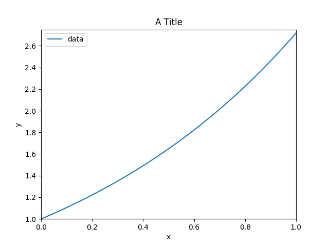
And the corresponding figure:

This is irritating for a few reasons. One is it is annoying to write python programs in string form; you don't get much editor support for indentation or syntax highlighting, and you have to be careful with quotes. It is not that easy to switch that snippet to Python mode either. You are pretty limited in writing programs that expand and modify the code too. Basically you have to do that all by string manipulation.

Along these lines, you could imagine a gnuplot function. It ends up not being much better.

(defun gnuplot (cmds)
  (let* ((temporary-file-directory ".")
         (cmdfile (make-temp-file "gnuplot-cmds-" nil ".gpl"))
         (shellcmd (format "gnuplot --persist -c \"%s\"" cmdfile)))
    (with-temp-file cmdfile
      (insert cmds))
    (shell-command shellcmd)
    (delete-file cmdfile)))

You use this the same way.

(gnuplot "set title \"Simple Plots\" font \",20\"
set key left box
set samples 50
set style data points
set terminal png
set output \"gnuplot.png\"

plot [-10:10] sin(x),atan(x),cos(atan(x))")

It has the same limitations as our string-based Python solution. The benefit of them is the native command structure for Python or gnuplot is used, so anything they can do you can too.

2 An alternative approach using a DSL

As an alternative, we consider here a domain specific language (DSL) that maps onto gnuplot. Suppose we could do this instead.

(gnuplot
 (set terminal png)
 (set output "test.png")
 (set title "Simple Plots" font ",20")
 (set key left box)
 (set samples 50)
 (set style data points)

 (plot [-10:10] sin\(x\) \,atan\(x\) \,cos\(atan\(x\)\)))

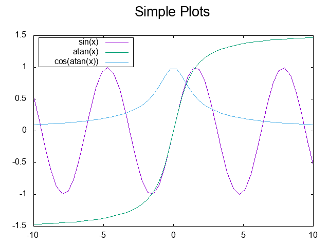
Here is the figure from that code. The most annoying part of this is in the plot function we have to escape all the parentheses and commas, but otherwise it looks pretty lispy. The output of that program is the gnuplot commands that were generated for making the plot.

This retains a lot of benefits of programming in lisp. gnuplot has to be a macro though because we do not want to evaluate the s-expressions inside as lisp. For starters they just look lispy, I don't actually use them as lisp at all. Instead we transform them to the gnuplot code.

In the following code, I will develop the gnuplot macro. It has some sticky and tricky points, and it is not obvious it will support all the features of gnuplot, but I learned a lot doing it that I will share here.

Starting with a simple form inside the macro, I wanted to convert (set output "test.png") to "set output \"test.png\"". For this DSL, I want to treat every symbol in the form as if it should be turned into a string, anything that is a string should be quoted, and anything that is in parentheses (i.e. it passes listp) should be evaluated and converted to a string. Then all those strings should be joined by spaces. Here is a macro that does that (adapted from a solution at https://emacs.stackexchange.com/questions/32558/eval-some-arguments-in-a-macro/32570?noredirect=1#comment50186_32570).

There are a couple of corner cases that are handled here. If the arg is a string, we quote it. If the arg is not a symbol or string, then it is evaluated and converted to a string. Importantly, this is done in the run environment though, so we can inject variables into the gnuplot code.

(defmacro gargs (&rest args)
  "Convert symbols to strings, quote strings, and (expr) to what they evaluate to."
  `(s-join " " (list ,@(cl-mapcan
                        (lambda (s)
                          (list
                           (cond
                            ((symbolp s)
                             (symbol-name s))
                            ((stringp s)
                             (format "\"%s\"" s))
                            (t
                             `(with-output-to-string
                                (princ ,s))))))
                        args))))

Here are a few examples of how it works. The loop is just to get a vertical table in org-mode for the blog post.

(loop for s in
      (list (gargs set key title "before fit" size \, (+ 5 5))
            (gargs set title "red")
            (gargs set yrange [0:*])
            (gargs "5")
            (let ((x 6)) (gargs (identity x)))
            (gargs 'x)
            (gargs '(x))
            (gargs set label 1 "plot for [n=2:10] sin(x*n)/n" at graph .95\, graph .92 right))
      collect
      (list s))

A limitation of this is that we either have quote things like parentheses, commas, semi-colons and sometimes square brackets:

(gargs plot for [n=2:10] sin\(x*n\)/n notitle lw \(13-n\)/2)

Or we have to use the string form instead; we can always fall back to that.

(gargs "plot for [n=2:10] sin(x*n)/n notitle lw (13-n)/2")

The macro above will do the grunt work on each form in the gnuplot macro. Finally, for the gnuplot macro, I want to take all the forms, convert them to gnuplot commands, write them to a temporary file, and then run gnuplot on the file, and finally delete the temp file. I assume we start with a gui terminal so graphs pop up unless you change it in your macro body. Here is that macro. It returns the generated code so it easy to see if you got the right program.

(defmacro gnuplot (&rest forms)
  (let* ((temporary-file-directory ".")
         (cmdfile (make-temp-file "gnuplot-cmds-" nil ".gpl"))
         (shellcmd (format "gnuplot --persist -c \"%s\"" cmdfile))
         (cmd-string))
    `(let ((cmd-string (s-join "\n" (list ,@(mapcar (lambda (x)
                                                      (if (stringp x)
                                                          x
                                                        `(gargs ,@x)))
                                                    forms)))))
       (with-temp-file ,cmdfile
         (insert "set terminal qt\n")
         (insert cmd-string)
         (setq cmd-string (buffer-string)))
       (shell-command ,shellcmd)
       (delete-file ,cmdfile)
       cmd-string)))

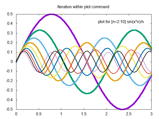
Here is a figure adapted from http://gnuplot.sourceforge.net/demo/iterate.html. I use the string form for the last line to avoid escaping all the special characters.

(gnuplot
 (set terminal png)
 (set output "iteration.png")
 (set title "Iteration within plot command")
 (set xrange [0:3])
 (set label 1 "plot for [n=2:10] sin(x*n)/n" at graph .95\, graph .92 right)
 "plot for [n=2:10] sin(x*n)/n notitle lw (13-n)/2")

Here is the resulting figure.

That is overall pretty sweet. There is a little dissonance between the strings, escaped comma, etc.., and it is not terribly ideal for integrating with regular lisp code inside the macro yet. That seems to be a feature of my choice to use (expr) as the syntax to evaluate a form. It means you have to do some gymnastics to get some s-expressions into the graphs. For example below I use a couple of variables to inject values. To get a string I have to use format to add the extra quotes, and to get the number I have to use the identity function. I also used escaped characters in the last line to see the difference.

(let ((ts "Iteration and substitution")
      (x0 0)
      (xf 3)
      (g1 0.95)
      (g2 0.92))
  (gnuplot
   (set terminal png)
   (set output "iteration-2.png")
   (set title (format "\"%s\"" ts))
   ;; Note the escaped square brackets
   (set xrange \[ (identity x0) : (identity xf) \])
   (set label 1 "plot for [n=2:10] sin(x*n)/n" at graph (identity g1) \, graph (identity g2) right)
   ;; note here I escaped the parentheses!
   (plot for [n=2:10] sin\(x*n\)/n notitle lw \(13-n\)/2)))

3 Summary

For the simple plots here, my DSL worked ok. There is a tradeoff in the syntax I chose that has some consequences. We cannot use the values of symbols in this DSL without resorting to hackery like (identity sym). We also cannot use the infix notation for sin(x) without quoting it as "sin(x)" or escaping the parentheses, e.g. sin\(x\), likewise square brackets which lisp will read as a vector. Commas have to be escaped, which is probably an emacs-lisp issue. To address that would require a reader macro which emacs-lisp does not have great support for. I am calling this experiment done for now. I have another syntax idea to try out another day.

Here is a preview of what it might look like. It is basically the same but I reuse keywords to indicate that :x0 should be replaced by whatever x0 evaluates to, and (: - 1 0.05) should be evaluated. The special character escaping is still there of course, since that is a limitation of the emacs lisp reader I think. I might try using x0? and (? - 1 0.05) instead. That might be less confusing. I like that the keywords are syntax highlighted for free though, and you can't use them for anything else.

(let ((ts "Iteration and substitution")
      (x0 0)
      (xf 3)
      (g2 0.92))
  (gnuplot
   (set terminal png)
   (set output "iteration-2.png")
   (set title :ts)
   ;; Note the escaped square brackets
   (set xrange \[ :x0 : :xf \])
   (set label 1 "plot for [n=2:10] sin(x*n)/n" at graph (: - 1 0.05) \, graph :g2 right)
   ;; note here I escaped the parentheses!
   (plot for [n=2:10] sin(x*n)/n notitle lw (13-n)/2)))

This has the benefit of a little cleaner injection of variables and selective execution of parenthetical expressions, we will just ignore any that don't pass (= (car expr) :). That May not work for sin((: + 1 1) x) though, unless I escape the outer parentheses too.

Copyright (C) 2017 by John Kitchin. See the License for information about copying.

org-mode source

Org-mode version = 9.0.5

Discuss on Twitter

Calling remote code-blocks in org-mode

| categories: orgmode, plotting, interactive | tags:

Table of Contents

We often write code in supporting information files that generates figures or tables in a scientific manuscript. Today, we explore how to call those code blocks remotely but get the output in the file we call it from. We will write code in si.org that generates an interactive figure that is presented in this file. We will use data published in hallenbeck-2015-compar-co2. You can find the data we used in the SI for that paper, or more conveniently here .

So, we make a named code block in the si.org file called "figure-1". Then we call it like this:

#+call: si.org:figure-1() :wrap html

That executes the code block in the other file, and wraps the output in an HTML block in this file! I do not like my code blocks to execute when I export because they are usually expensive calculations, so I have to manually run the line with C-c C-c, but you can override that behavior with a local setting of org-export-babel-evaluate. So, without further delay, here is the result. Now we have a nice, neat blog post file, with code in an si.org file!

Copyright (C) 2016 by John Kitchin. See the License for information about copying.

org-mode source

Org-mode version = 8.2.10

Discuss on Twitter

Interactive figures in blog posts with mpld3

| categories: plotting, interactive, python | tags:

Continuing the exploration of interactive figures, today we consider the Python plotting library mpld3 . We will again use our own published data. We wrote this great paper on core level shifts (CLS) in Cu-Pd alloys boes-2015-core-cu. I want an interactive figure that shows the name of the calculation on each point as a tooltip. This data is all stored in the supporting information file, and you can see how we use it here. This figure shows how the core level shift of a Cu atom changes depending on the number of nearest neighbor Cu atoms. Just hover your mouse over a point to see the name and CLS for that point.

1 Data and code

You can check out our preprint at https://github.com/KitchinHUB/kitchingroup-51 . We are going to adapt the code to make Figure 6a in the manuscript interactive. The code needed a somewhat surprising amount of adaptation. Apparently the ase database interface has changed a lot since we write that paper, so the code here looks a bit different than what we published. The biggest difference is due to name-mangling so each key that started with a number now starts with _, and and periods are replaced by _ also. The rest of the script is nearly unchanged. At the end is the very small bit of mpld3 code that generates the figure for html. We will add tooltips onto datapoints to indicate what the name associated with each data point is. Here is the code.

import matplotlib.pyplot as plt
from ase.db import connect

# loads the ASE database and select certain keywords
db = connect('~/Desktop/cappa/kitchingroup-51/supporting-information/data.json')

keys = ['bcc', 'GS', '_54atom', 'ensam']

CLS, IMP, labels = [], [], []
for k in db.select(keys + ['_1cl']):
    name = k.keywords[-2]

    Cu0 = db.select('bcc,GS,_72atom,_0cl,_1_00Cu').next().energy
    Cu1 = db.select('bcc,GS,_72atom,_1cl,_1_00Cu').next().energy
    x0 = db.select(','.join(keys + [name, '_0cl'])).next().energy
    x1 = k.energy

    cls0 = x0 - Cu0
    cls1 = x1 - Cu1

    IMP.append(int(name[1]))
    CLS.append(cls1 - cls0)
    labels += ['{0} ({1}, {2})'.format(name, int(name[1]), cls1 - cls0)]

Cu0 = db.select(','.join(['bcc', 'GS', '_72atom',
                          '_0cl', '_1_00Cu'])).next().energy
Cu1 = db.select(','.join(['bcc', 'GS', '_72atom',
                          '_1cl', '_1_00Cu'])).next().energy

x0 = db.select(','.join(['bcc', 'GS', '_54atom',
                         '_0cl', '_1'])).next().energy
x1 = db.select(','.join(['bcc', 'GS', '_54atom',
                         '_1cl', '_1'])).next().energy

cls0 = x0 - Cu0
cls1 = x1 - Cu1

IMP.append(1)
CLS.append(cls1 - cls0)
labels += ['(1, {0})'.format(cls1 - cls0)]

Cu0 = db.select(','.join(['bcc', 'GS', '_72atom',
                          '_0cl', '_1_00Cu'])).next().energy
Cu1 = db.select(','.join(['bcc', 'GS', '_72atom',
                          '_1cl', '_1_00Cu'])).next().energy

x0 = db.select(','.join(['bcc', 'GS', '_54atom',
                         '_0cl', '_0'])).next().energy
x1 = db.select(','.join(['bcc', 'GS', '_54atom',
                         '_1cl', '_0'])).next().energy

cls0 = x0 - Cu0
cls1 = x1 - Cu1

IMP.append(0)
CLS.append(cls1 - cls0)
labels += ['(0, {0})'.format(cls1 - cls0)]

fig = plt.figure()

p = plt.scatter(IMP, CLS, c='g', marker='o', s=25)
ax1 = plt.gca()
ax1.set_ylim(-1.15, -0.6)
ax1.set_xlim(-0.1, 5.1)

ax1.set_xlabel('# Cu Nearest neighbors')
ax1.set_ylabel('Cu 2p(3/2) Core Level Shift (eV)')

ax1.set_title('Hover over a point to see the calculation name')

# Now the mpld3 stuff.
import mpld3
from mpld3 import plugins

tooltip = plugins.PointHTMLTooltip(p, labels, voffset=0, hoffset=10)
plugins.connect(fig, tooltip)

print mpld3.fig_to_html(fig)

I like this workflow pretty well. It seems less functional than plotly and Bokeh (e.g. it does not look like it you can export the data from the html here), but it is well integrated with Matplotlib, with my blogging style, and does not require a server, oran account. The code outputs html that is self-contained in the body of the html. The smooth integration with Matplotlib means I could have static images in org-mode, and dynamic images in HTML potentially. Overall, this is a nice tool for making interactive plots in blog posts.

Copyright (C) 2016 by John Kitchin. See the License for information about copying.

org-mode source

Org-mode version = 8.2.10

Discuss on Twitter

Interactive Bokeh plots in HTML

| categories: plotting, interactive, python | tags:

In our last post we examined the use of plotly to generate interactive plots in HTML. Today we expand the idea, and use Bokeh . One potential issue with plotly is the need for an account and API-key, some limitations on how many times a graph can be viewed per day (although I should aspire to have my graphs viewed 1000+ times a day!), and who knows what happens to the graphs if plotly ever goes out of business. While the static images we usually use have limited utility, at least they stick around.

So, today we look at Bokeh which allows you to embed some json data in your HTML, which is made interactive by your browser with more javascript magic. We get straight to the image here so you can see what this is all about. Briefly, this data shows trends (or lack of) in the adsorption energies of some atoms on the atop and fcc sites of several transition metals as a function of adsorbate coverage xu-2014-probin-cover. The code to do this is found here.

Using Bokeh does not integrate real smoothly with my blog workflow, which only generates the body of HTML posts. Bokeh needs some javascript injected into the header to work. To get around that, I show the plot in a frame here. You can see a full HTML version here: bokeh-plot.html .

This is somewhat similar to the plotly concept. The data is embedded in the html in this case, which is different. For very large plots, I actually had some trouble exporting the blog post (it was taking a long time to export and I killed it)! I suspect that is a limitation of the org-mode exporter though, because I could save the html files from Python and view them fine. I also noted that having all the javascript in the org-file make font-lock work very slow. It would be better to generate that only on export.

Note to make this work, we need these lines in our HTML header:

#+HTML_HEAD: <link rel="stylesheet" href="http://cdn.pydata.org/bokeh/release/bokeh-0.11.1.min.css" type="text/css" />
#+HTML_HEAD: <script type="text/javascript" src="http://cdn.pydata.org/bokeh/release/bokeh-0.11.1.min.js"></script>

Since we do not host those locally, if they ever disappear, our plots will not show ;(

1 The data and code

We will get the data from our paper on coverage dependent adsorption energies xu-2014-probin-cover. There are some data rich figures there that would benefit from some interactivity. You can get the data here: http://pubs.acs.org/doi/suppl/10.1021/jp508805h . Extract out the supporting-information.org and energies.json file to follow here. We will make Figure 2a in the SI document here, and make it interactive with hover tooltips.

import json

from collections import OrderedDict
from bokeh import mpl
from bokeh.plotting import *
from bokeh.models import HoverTool
from bokeh.embed import components

with open('/users/jkitchin/Desktop/energies.json', 'r') as f:
    data = json.load(f)


# color for metal
# letter symbol for adsorbate
colors = {'Cu':'Orange',
          'Ag':'Silver',
          'Au':'Yellow',
          'Pd':'Green',
          'Pt':'Red',
          'Rh':'Blue',
          'Ir':'Purple'}

all_ads = ['O', 'S']

TOOLS="crosshair,pan,wheel_zoom,box_zoom,reset,hover,previewsave"
p = figure(title="Correlation between atop and fcc sites", tools=TOOLS)

for metal in ['Rh', 'Pd', 'Cu', 'Ag']:
    for adsorbate in all_ads:
        E1, E2 = [], []
        for coverage in '0.25', '0.5', '0.75', '1.0':
            if (isinstance(data[metal][adsorbate]['ontop'][coverage], float) and
                isinstance(data[metal][adsorbate]['fcc'][coverage], float)):
                E1.append(data[metal][adsorbate]['ontop'][coverage])
                E2.append(data[metal][adsorbate]['fcc'][coverage])
        labels = ['{0}-{1} {2} ML'.format(metal, adsorbate, x)
                  for x in ['0.25', '0.5', '0.75', '1.0']]
        p.line('x', 'y', color=colors[metal],
               source=ColumnDataSource(data={'x': E1,
                                             'y': E2,
                                             'label': labels}))
        p.circle('x', 'y', color=colors[metal],
               source=ColumnDataSource(data={'x': E1,
                                             'y': E2,
                                             'label': labels}))


hover =p.select({'type': HoverTool})
hover.tooltips = OrderedDict([("(atop,fcc)", "(@x, @y)"),
                              ("label", "@label")])

p.xaxis.axis_label = 'Adsorption energy on the atop site'
p.yaxis.axis_label = 'Adsorption energy on the fcc site'

script, div = components(p)
script = '\n'.join(['#+HTML_HEAD_EXTRA: ' + line for line in script.split('\n')])

print '''{script}

#+BEGIN_HTML
<a name="figure"></a>
{div}
#+END_HTML
'''.format(script=script, div=div)

Copyright (C) 2016 by John Kitchin. See the License for information about copying.

org-mode source

Org-mode version = 8.2.10

Discuss on Twitter
Next Page »