Vectorized piecewise functions

| categories: math | tags:

Matlab post Occasionally we need to define piecewise functions, e.g.

\begin{eqnarray} f(x) &=& 0, x < 0 \\ &=& x, 0 <= x < 1\\ &=& 2 - x, 1 < x <= 2\\ &=& 0, x > 2 \end{eqnarray}

Today we examine a few ways to define a function like this. A simple way is to use conditional statements.

def f1(x):
    if x < 0:
        return 0
    elif (x >= 0) & (x < 1):
        return x
    elif (x >= 1) & (x < 2):
        return 2.0 - x
    else:
        return 0

print f1(-1)
print f1([0, 1, 2, 3])  # does not work!
... ... ... ... ... ... ... ... >>> 0
0

This works, but the function is not vectorized, i.e. f([-1 0 2 3]) does not evaluate properly (it should give a list or array). You can get vectorized behavior by using list comprehension, or by writing your own loop. This does not fix all limitations, for example you cannot use the f1 function in the quad function to integrate it.

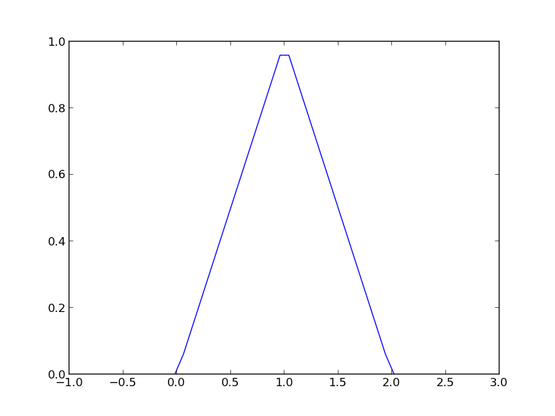
import numpy as np
import matplotlib.pyplot as plt

x = np.linspace(-1, 3)
y = [f1(xx) for xx in x]

plt.plot(x, y)
plt.savefig('images/vector-piecewise.png')
>>> >>> >>> >>> >>> [<matplotlib.lines.Line2D object at 0x048D6790>]

Neither of those methods is convenient. It would be nicer if the function was vectorized, which would allow the direct notation f1([0, 1, 2, 3, 4]). A simple way to achieve this is through the use of logical arrays. We create logical arrays from comparison statements.

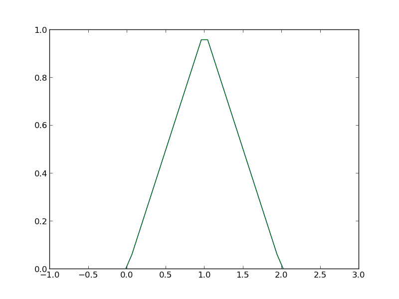
def f2(x):
    'fully vectorized version'
    x = np.asarray(x)
    y = np.zeros(x.shape)
    y += ((x >= 0) & (x < 1)) * x
    y += ((x >= 1) & (x < 2)) * (2 - x)
    return y

print f2([-1, 0, 1, 2, 3, 4])
x = np.linspace(-1,3);
plt.plot(x,f2(x))
plt.savefig('images/vector-piecewise-2.png')
... ... ... ... ... ... >>> [ 0.  0.  1.  0.  0.  0.]
>>> [<matplotlib.lines.Line2D object at 0x043A4910>]

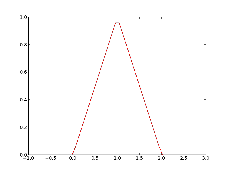
A third approach is to use Heaviside functions. The Heaviside function is defined to be zero for x less than some value, and 0.5 for x=0, and 1 for x >= 0. If you can live with y=0.5 for x=0, you can define a vectorized function in terms of Heaviside functions like this.

def heaviside(x):
    x = np.array(x)
    if x.shape != ():
        y = np.zeros(x.shape)
        y[x > 0.0] = 1
        y[x == 0.0] = 0.5
    else: # special case for 0d array (a number)
        if x > 0: y = 1
        elif x == 0: y = 0.5
        else: y = 0
    return y

def f3(x):
    x = np.array(x)
    y1 = (heaviside(x) - heaviside(x - 1)) * x # first interval
    y2 = (heaviside(x - 1) - heaviside(x - 2)) * (2 - x) # second interval
    return y1 + y2

from scipy.integrate import quad
print quad(f3, -1, 3)
... ... ... ... ... ... ... ... ... ... >>> ... ... ... ... ... >>> >>> (1.0, 1.1102230246251565e-14)
plt.plot(x, f3(x))
plt.savefig('images/vector-piecewise-3.png')
[<matplotlib.lines.Line2D object at 0x048F96F0>]

There are many ways to define piecewise functions, and vectorization is not always necessary. The advantages of vectorization are usually notational simplicity and speed; loops in python are usually very slow compared to vectorized functions.

Copyright (C) 2013 by John Kitchin. See the License for information about copying.

org-mode source

Discuss on Twitter

The trapezoidal method of integration

| categories: integration, math | tags:

Matlab post See http://en.wikipedia.org/wiki/Trapezoidal_rule

$$\int_a^b f(x) dx \approx \frac{1}{2}\displaystyle\sum\limits_{k=1}^N(x_{k+1}-x_k)(f(x_{k+1}) + f(x_k))$$

Let us compute the integral of sin(x) from x=0 to \(\pi\). To approximate the integral, we need to divide the interval from \(a\) to \(b\) into \(N\) intervals. The analytical answer is 2.0.

We will use this example to illustrate the difference in performance between loops and vectorized operations in python.

import numpy as np
import time

a = 0.0; b = np.pi;
N = 1000; # this is the number of intervals

h = (b - a)/N; # this is the width of each interval
x = np.linspace(a, b, N) 
y = np.sin(x); # the sin function is already vectorized

t0 = time.time()
f = 0.0
for k in range(len(x) - 1):
    f += 0.5 * ((x[k+1] - x[k]) * (y[k+1] + y[k]))

tf = time.time() - t0
print 'time elapsed = {0} sec'.format(tf)

print f
>>> >>> >>> >>> >>> >>> >>> >>> >>> >>> >>> ... ... >>> >>> time elapsed = 0.0780000686646 sec
>>> 1.99999835177
t0 = time.time()
Xk = x[1:-1] - x[0:-2] # vectorized version of (x[k+1] - x[k])
Yk = y[1:-1] + y[0:-2] # vectorized version of (y[k+1] + y[k])

f = 0.5 * np.sum(Xk * Yk) # vectorized version of the loop above
tf = time.time() - t0
print 'time elapsed = {0} sec'.format(tf)

print f
>>> >>> >>> >>> >>> time elapsed = 0.077999830246 sec
>>> 1.99999340709

In the last example, there may be loop buried in the sum command. Let us do one final method, using linear algebra, in a single line. The key to understanding this is to recognize the sum is just the result of a dot product of the x differences and y sums.

t0 = time.time()
f = 0.5 * np.dot(Xk, Yk)
tf = time.time() - t0
print 'time elapsed = {0} sec'.format(tf)

print f
>>> >>> time elapsed = 0.0310001373291 sec
>>> 1.99999340709

The loop method is straightforward to code, and looks alot like the formula that defines the trapezoid method. the vectorized methods are not as easy to read, and take fewer lines of code to write. However, the vectorized methods are much faster than the loop, so the loss of readability could be worth it for very large problems.

The times here are considerably slower than in Matlab. I am not sure if that is a totally fair comparison. Here I am running python through emacs, which may result in slower performance. I also used a very crude way of timing the performance which lumps some system performance in too.

Copyright (C) 2013 by John Kitchin. See the License for information about copying.

org-mode source

Discuss on Twitter

Phase portraits of a system of ODEs

| categories: math, ode | tags:

Matlab post An undamped pendulum with no driving force is described by

$$ y'' + sin(y) = 0$$

We reduce this to standard matlab form of a system of first order ODEs by letting \(y_1 = y\) and \(y_2=y_1'\). This leads to:

\(y_1' = y_2\)

\(y_2' = -sin(y_1)\)

The phase portrait is a plot of a vector field which qualitatively shows how the solutions to these equations will go from a given starting point. here is our definition of the differential equations:

To generate the phase portrait, we need to compute the derivatives \(y_1'\) and \(y_2'\) at \(t=0\) on a grid over the range of values for \(y_1\) and \(y_2\) we are interested in. We will plot the derivatives as a vector at each (y1, y2) which will show us the initial direction from each point. We will examine the solutions over the range -2 < y1 < 8, and -2 < y2 < 2 for y2, and create a grid of 20 x 20 points.

import numpy as np
import matplotlib.pyplot as plt

def f(Y, t):
    y1, y2 = Y
    return [y2, -np.sin(y1)]

y1 = np.linspace(-2.0, 8.0, 20)
y2 = np.linspace(-2.0, 2.0, 20)

Y1, Y2 = np.meshgrid(y1, y2)

t = 0

u, v = np.zeros(Y1.shape), np.zeros(Y2.shape)

NI, NJ = Y1.shape

for i in range(NI):
    for j in range(NJ):
        x = Y1[i, j]
        y = Y2[i, j]
        yprime = f([x, y], t)
        u[i,j] = yprime[0]
        v[i,j] = yprime[1]
     

Q = plt.quiver(Y1, Y2, u, v, color='r')

plt.xlabel('$y_1$')
plt.ylabel('$y_2$')
plt.xlim([-2, 8])
plt.ylim([-4, 4])
plt.savefig('images/phase-portrait.png')
>>> ... >>> >>> >>> >>> >>> >>> ... ... ... >>> >>> <matplotlib.text.Text object at 0xbcfd290>
<matplotlib.text.Text object at 0xbd14750>
(-2, 8)
(-4, 4)

Let us plot a few solutions on the vector field. We will consider the solutions where y1(0)=0, and values of y2(0) = [0 0.5 1 1.5 2 2.5], in otherwords we start the pendulum at an angle of zero, with some angular velocity.

from scipy.integrate import odeint

for y20 in [0, 0.5, 1, 1.5, 2, 2.5]:
    tspan = np.linspace(0, 50, 200)
    y0 = [0.0, y20]
    ys = odeint(f, y0, tspan)
    plt.plot(ys[:,0], ys[:,1], 'b-') # path
    plt.plot([ys[0,0]], [ys[0,1]], 'o') # start
    plt.plot([ys[-1,0]], [ys[-1,1]], 's') # end
    

plt.xlim([-2, 8])
plt.savefig('images/phase-portrait-2.png')
plt.show()
>>> ... ... ... [<matplotlib.lines.Line2D object at 0xbc0dbd0>]
[<matplotlib.lines.Line2D object at 0xc135050>]
[<matplotlib.lines.Line2D object at 0xbd1a450>]
[<matplotlib.lines.Line2D object at 0xbd1a1d0>]
[<matplotlib.lines.Line2D object at 0xb88aa10>]
[<matplotlib.lines.Line2D object at 0xb88a5d0>]
[<matplotlib.lines.Line2D object at 0xc14e410>]
[<matplotlib.lines.Line2D object at 0xc14ed90>]
[<matplotlib.lines.Line2D object at 0xc2c5290>]
[<matplotlib.lines.Line2D object at 0xbea4bd0>]
[<matplotlib.lines.Line2D object at 0xbea4d50>]
[<matplotlib.lines.Line2D object at 0xbc401d0>]
[<matplotlib.lines.Line2D object at 0xc2d1190>]
[<matplotlib.lines.Line2D object at 0xc2f3e90>]
[<matplotlib.lines.Line2D object at 0xc2f3bd0>]
[<matplotlib.lines.Line2D object at 0xc2e4790>]
[<matplotlib.lines.Line2D object at 0xc2e0a90>]
[<matplotlib.lines.Line2D object at 0xc2c7390>]
(-2, 8)

What do these figures mean? For starting points near the origin, and small velocities, the pendulum goes into a stable limit cycle. For others, the trajectory appears to fly off into y1 space. Recall that y1 is an angle that has values from \(-\pi\) to \(\pi\). The y1 data in this case is not wrapped around to be in this range.

Copyright (C) 2013 by John Kitchin. See the License for information about copying.

org-mode source

Discuss on Twitter

Random thoughts

| categories: math, statistics | tags:

Matlab post

Random numbers are used in a variety of simulation methods, most notably Monte Carlo simulations. In another later example, we will see how we can use random numbers for error propagation analysis. First, we discuss two types of pseudorandom numbers we can use in python: uniformly distributed and normally distributed numbers.

Say you are the gambling type, and bet your friend $5 the next random number will be greater than 0.49. Let us ask Python to roll the random number generator for us.

import numpy as np

n = np.random.uniform()
print 'n = {0}'.format(n)

if n > 0.49:
    print 'You win!'
else:
    print 'you lose.'
n = 0.381896986693
you lose.

The odds of you winning the last bet are slightly stacked in your favor. There is only a 49% chance your friend wins, but a 51% chance that you win. Lets play the game a lot of times times and see how many times you win, and your friend wins. First, lets generate a bunch of numbers and look at the distribution with a histogram.

import numpy as np

N = 10000
games = np.random.uniform(size=(1,N))

wins = np.sum(games > 0.49)
losses = N - wins

print 'You won {0} times ({1:%})'.format(wins, float(wins) / N)

import matplotlib.pyplot as plt
count, bins, ignored = plt.hist(games)
plt.savefig('images/random-thoughts-1.png')
You won 5090 times (50.900000%)

As you can see you win slightly more than you lost.

It is possible to get random integers. Here are a few examples of getting a random integer between 1 and 100. You might do this to get random indices of a list, for example.

import numpy as np

print np.random.random_integers(1, 100)
print np.random.random_integers(1, 100, 3)
print np.random.random_integers(1, 100, (2,2))
96
[ 95  49 100]
[[69 54]
 [41 93]]

The normal distribution is defined by \(f(x)=\frac{1}{\sqrt{2\pi \sigma^2}} \exp (-\frac{(x-\mu)^2}{2\sigma^2})\) where \(\mu\) is the mean value, and \(\sigma\) is the standard deviation. In the standard distribution, \(\mu=0\) and \(\sigma=1\).

import numpy as np

mu = 1
sigma = 0.5
print np.random.normal(mu, sigma)
print np.random.normal(mu, sigma, 2)
1.04225842065
[ 0.58105204  0.64853157]

Let us compare the sampled distribution to the analytical distribution. We generate a large set of samples, and calculate the probability of getting each value using the matplotlib.pyplot.hist command.

import numpy as np
import matplotlib.pyplot as plt

mu = 0; sigma = 1

N = 5000
samples = np.random.normal(mu, sigma, N)

counts, bins, ignored = plt.hist(samples, 50, normed=True)

plt.plot(bins, 1.0/np.sqrt(2 * np.pi * sigma**2)*np.exp(-((bins - mu)**2)/(2*sigma**2)))
plt.savefig('images/random-thoughts-2.png')

What fraction of points lie between plus and minus one standard deviation of the mean?

samples >= mu-sigma will return a vector of ones where the inequality is true, and zeros where it is not. (samples >= mu-sigma) & (samples <= mu+sigma) will return a vector of ones where there is a one in both vectors, and a zero where there is not. In other words, a vector where both inequalities are true. Finally, we can sum the vector to get the number of elements where the two inequalities are true, and finally normalize by the total number of samples to get the fraction of samples that are greater than -sigma and less than sigma.

import numpy as np
import matplotlib.pyplot as plt

mu = 0; sigma = 1

N = 5000
samples = np.random.normal(mu, sigma, N)

a = np.sum((samples >= (mu - sigma)) & (samples <= (mu + sigma))) / float(N) 
b = np.sum((samples >= (mu - 2*sigma)) & (samples <= (mu + 2*sigma))) / float(N) 
print '{0:%} of samples are within +- standard deviations of the mean'.format(a)
print '{0:%} of samples are within +- 2standard deviations of the mean'.format(b)
67.500000% of samples are within +- standard deviations of the mean
95.580000% of samples are within +- 2standard deviations of the mean

1 Summary

We only considered the numpy.random functions here, and not all of them. There are many distributions of random numbers to choose from. There are also random numbers in the python random module. Remember these are only pseudorandom numbers, but they are still useful for many applications.

Copyright (C) 2013 by John Kitchin. See the License for information about copying.

org-mode source

Discuss on Twitter

Solving Bessel's Equation numerically

| categories: math, ode | tags:

Matlab post

Reference Ch 5.5 Kreysig, Advanced Engineering Mathematics, 9th ed.

Bessel's equation \(x^2 y'' + x y' + (x^2 - \nu^2)y=0\) comes up often in engineering problems such as heat transfer. The solutions to this equation are the Bessel functions. To solve this equation numerically, we must convert it to a system of first order ODEs. This can be done by letting \(z = y'\) and \(z' = y''\) and performing the change of variables:

$$ y' = z$$

$$ z' = \frac{1}{x^2}(-x z - (x^2 - \nu^2) y$$

if we take the case where \(\nu = 0\), the solution is known to be the Bessel function \(J_0(x)\), which is represented in Matlab as besselj(0,x). The initial conditions for this problem are: \(y(0) = 1\) and \(y'(0)=0\).

There is a problem with our system of ODEs at x=0. Because of the \(1/x^2\) term, the ODEs are not defined at x=0. If we start very close to zero instead, we avoid the problem.

import numpy as np
from scipy.integrate import odeint
from scipy.special import jn # bessel function
import matplotlib.pyplot as plt

def fbessel(Y, x):
    nu = 0.0
    y = Y[0]
    z = Y[1]
  
    dydx = z
    dzdx = 1.0 / x**2 * (-x * z - (x**2 - nu**2) * y)
    return [dydx, dzdx]

x0 = 1e-15
y0 = 1
z0 = 0
Y0 = [y0, z0]

xspan = np.linspace(1e-15, 10)
sol = odeint(fbessel, Y0, xspan)

plt.plot(xspan, sol[:,0], label='numerical soln')
plt.plot(xspan, jn(0, xspan), 'r--', label='Bessel')
plt.legend()
plt.savefig('images/bessel.png')

You can see the numerical and analytical solutions overlap, indicating they are at least visually the same.

Copyright (C) 2013 by John Kitchin. See the License for information about copying.

org-mode source

Discuss on Twitter
« Previous Page -- Next Page »