Visualizing uncertainty in linear regression

| categories: data analysis, uncertainty | tags:

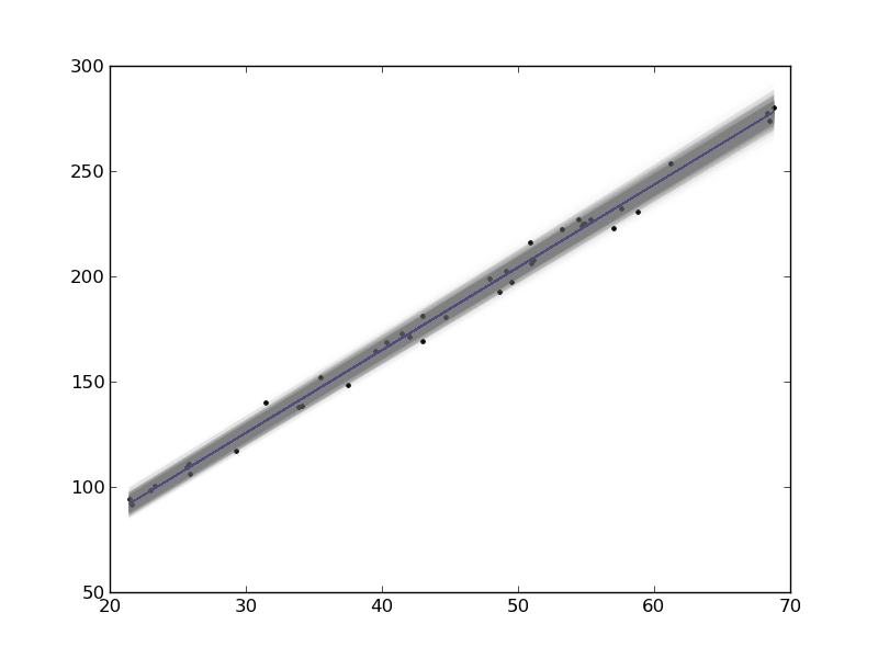
In this example, we show how to visualize uncertainty in a fit. The idea is to fit a model to data, and get the uncertainty in the model parameters. Then we sample the parameters according to the normal distribution, and plot the corresponding distribution of models. We use transparent lines and allow the overlap to indicate the density of the fits.

The data is stored in a text file download PT.txt , with the following structure:

Run          Ambient                            Fitted
 Order  Day  Temperature  Temperature  Pressure    Value    Residual
  1      1      23.820      54.749      225.066   222.920     2.146
...

We need to read the data in, and perform a regression analysis on P vs. T. In python we start counting at 0, so we actually want columns 3 and 4.

import numpy as np
import matplotlib.pyplot as plt
from pycse import regress

data = np.loadtxt('../../pycse/data/PT.txt', skiprows=2)
T = data[:, 3]
P = data[:, 4]

A = np.column_stack([T**0, T])

p, pint, se = regress(A, P, 0.05)

print p, pint, se
plt.plot(T, P, 'k.')
plt.plot(T, np.dot(A, p))

# Now we plot the distribution of possible lines
N = 2000
B = np.random.normal(p[0], se[0], N)
M = np.random.normal(p[1], se[1], N)
x = np.array([min(T), max(T)])

for b,m in zip(B, M):
    plt.plot(x, m*x + b, '-', color='gray', alpha=0.02)
plt.savefig('images/plotting-uncertainty.png')
[ 7.74899739  3.93014044] [[  2.97964903  12.51834576]
 [  3.82740876   4.03287211]] [ 2.35384765  0.05070183]

Here you can see 2000 different lines that have some probability of being correct. The darkest gray is near the fit, as expected; the darker the gray the more probable it is the line. This is a qualitative way of judging the quality of the fit.

Note, this is not the prediction error that we are plotting, that is the uncertainty in where a predicted y-value is.

Copyright (C) 2013 by John Kitchin. See the License for information about copying.

org-mode source
Discuss on Twitter

Uncertainty in polynomial roots - Part II

| categories: data analysis, uncertainty | tags:

We previously looked at uncertainty in polynomial roots where we had an analytical formula for the roots of the polynomial, and we knew the uncertainties in the polynomial parameters. It would be inconvenient to try this for a cubic polynomial, although there may be formulas for the roots. I do not know of there are general formulas for the roots of a 4th order polynomial or higher.

Unfortunately, we cannot use the uncertainties package out of the box directly here.

import uncertainties as u
import numpy as np
c, b, a = [-0.99526746, -0.011546,    1.00188999]
sc, sb, sa = [ 0.0249142,   0.00860025,  0.00510128]

A = u.ufloat((a, sa))
B = u.ufloat((b, sb))
C = u.ufloat((c, sc))

print np.roots([A, B, C])
>>> >>> >>> >>> >>> >>> >>> >>> Traceback (most recent call last):
  File "<stdin>", line 1, in <module>
  File "c:\Users\jkitchin\AppData\Local\Enthought\Canopy\User\lib\site-packages\numpy\lib\polynomial.py", line 218, in roots
    p = p.astype(float)
  File "c:\Users\jkitchin\AppData\Local\Enthought\Canopy\User\lib\site-packages\uncertainties\__init__.py", line 1257, in raise_error
    % (self.__class__, coercion_type))
TypeError: can't convert an affine function (<class 'uncertainties.Variable'>) to float; use x.nominal_value

To make some progress, we have to understand how the numpy.roots function works. It constructs a Companion matrix, and the eigenvalues of that matrix are the same as the roots of the polynomial.

import numpy as np

c0, c1, c2 = [-0.99526746, -0.011546,    1.00188999]

p = np.array([c2, c1, c0])
N = len(p)

# we construct the companion matrix like this
# see https://github.com/numpy/numpy/blob/v1.7.0/numpy/lib/polynomial.py#L220
# for this code.
# build companion matrix and find its eigenvalues (the roots)
A = np.diag(np.ones((N-2,), p.dtype), -1)
A[0, :] = -p[1:] / p[0]

print A

roots = np.linalg.eigvals(A)
print roots
[[ 0.01152422  0.99338996]
 [ 1.          0.        ]]
[ 1.00246827 -0.99094405]

This definition of the companion matrix is a little different than the one here, but primarily in the scaling of the coefficients. That does not seem to change the eigenvalues, or the roots.

Now, we have a path to estimate the uncertainty in the roots. Since we know the polynomial coefficients and their uncertainties from the fit, we can use Monte Carlo sampling to estimate the uncertainty in the roots.

import numpy as np
import uncertainties as u

c, b, a = [-0.99526746, -0.011546,    1.00188999]
sc, sb, sa = [ 0.0249142,   0.00860025,  0.00510128]

NSAMPLES = 100000
A = np.random.normal(a, sa, (NSAMPLES, ))
B = np.random.normal(b, sb, (NSAMPLES, ))
C = np.random.normal(c, sc, (NSAMPLES, ))

roots = [[] for i in range(NSAMPLES)]

for i in range(NSAMPLES):
    p = np.array([A[i], B[i], C[i]])
    N = len(p)
    
    M = np.diag(np.ones((N-2,), p.dtype), -1)
    M[0, :] = -p[1:] / p[0]
    r = np.linalg.eigvals(M)
    r.sort()  # there is no telling what order the values come out in
    roots[i] = r
    
avg = np.average(roots, axis=0)
std = np.std(roots, axis=0)

for r, s in zip(avg, std):
    print '{0: f} +/- {1: f}'.format(r, s)
-0.990949 +/-  0.013435
 1.002443 +/-  0.013462

Compared to our previous approach with the uncertainties package where we got:

: -0.990944048037+/-0.0134208013339
:  1.00246826738 +/-0.0134477390832

the agreement is quite good! The advantage of this approach is that we do not have to know the formula for the roots of higher order polynomials to estimate the uncertainty in the roots. The downside is we have to evaluate the eigenvalues of a matrix a large number of times to get good estimates of the uncertainty. For high power polynomials this could be problematic. I do not currently see a way around this, unless it becomes possible to get the uncertainties package to propagate through the numpy.eigvals function. It is possible to wrap some functions with uncertainties, but so far only functions that return a single number.

There are some other potential problems with this approach. It is assumed that the accuracy of the eigenvalue solver is much better than the uncertainty in the polynomial parameters. You have to use some judgment in using these uncertainties. We are approximating the uncertainties of a nonlinear problem. In other words, the uncertainties of the roots are not linearly dependent on the uncertainties of the polynomial coefficients.

It is possible to wrap some functions with uncertainties, but so far only functions that return a single number. Here is an example of getting the nth root and its uncertainty.

import uncertainties as u
import numpy as np

@u.wrap
def f(n=0, *P):
    ''' compute the nth root of the polynomial P and the uncertainty of the root'''
    p =  np.array(P)
    N = len(p)
    
    M = np.diag(np.ones((N-2,), p.dtype), -1)
    M[0, :] = -p[1:] / p[0]
    r = np.linalg.eigvals(M)
    r.sort()  # there is no telling what order the values come out in
    return r[n]

# our polynomial coefficients and standard errors
c, b, a = [-0.99526746, -0.011546,    1.00188999]
sc, sb, sa = [ 0.0249142,   0.00860025,  0.00510128]

A = u.ufloat((a, sa))
B = u.ufloat((b, sb))
C = u.ufloat((c, sc))

for result in [f(n, A, B, C) for n in [0, 1]]:
    print result
-0.990944048037+/-0.013420800377
1.00246826738+/-0.0134477388218

It is good to see this is the same result we got earlier, with a lot less work (although we do have to solve it for each root, which is a bit redundant)! It is a bit more abstract though, and requires a specific formulation of the function for the wrapper to work.

Copyright (C) 2013 by John Kitchin. See the License for information about copying.

org-mode source
Discuss on Twitter

Uncertainty in polynomial roots

| categories: data analysis, uncertainty | tags:

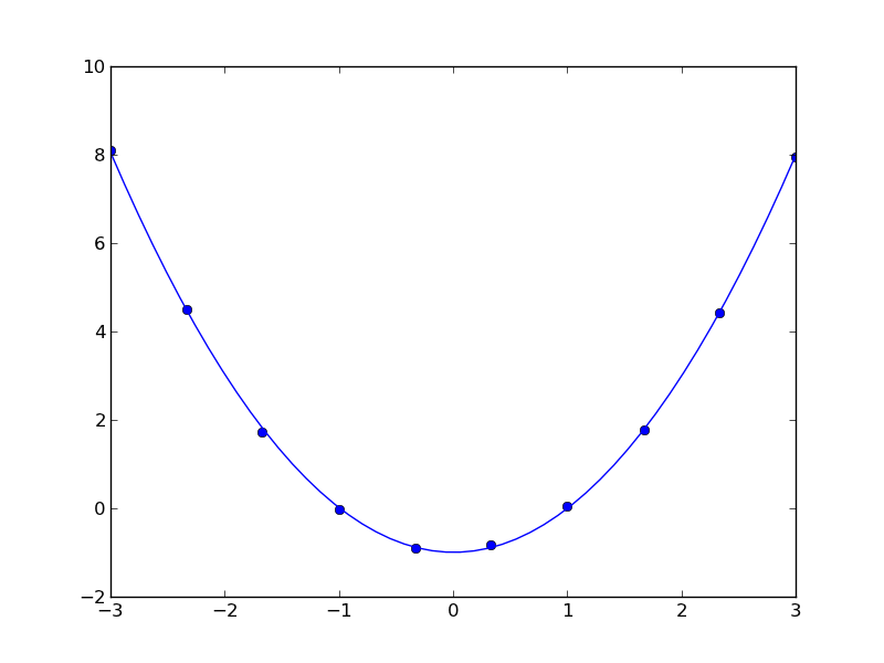
Polynomials are convenient for fitting to data. Frequently we need to derive some properties of the data from the fit, e.g. the minimum value, or the slope, etc… Since we are fitting data, there is uncertainty in the polynomial parameters, and corresponding uncertainty in any properties derived from those parameters.

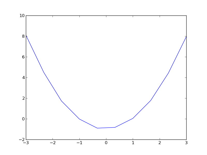
Here is our data.

-3.00 8.10
-2.33 4.49
-1.67 1.73
-1.00 -0.02
-0.33 -0.90
0.33 -0.83
1.00 0.04
1.67 1.78
2.33 4.43
3.00 7.95
import matplotlib.pyplot as plt

x = [a[0] for a in data]
y = [a[1] for a in data]
plt.plot(x, y)
plt.savefig('images/uncertain-roots.png')

import matplotlib.pyplot as plt
import numpy as np
from pycse import regress

x = np.array([a[0] for a in data])
y = [a[1] for a in data]

A = np.column_stack([x**0, x**1, x**2])

p, pint, se = regress(A, y, alpha=0.05)

print p

print pint

print se

plt.plot(x, y, 'bo ')

xfit = np.linspace(x.min(), x.max())
plt.plot(xfit, np.dot(np.column_stack([xfit**0, xfit**1, xfit**2]), p), 'b-')
plt.savefig('images/uncertain-roots-1.png')
[-0.99526746 -0.011546    1.00188999]
[[-1.05418017 -0.93635474]
 [-0.03188236  0.00879037]
 [ 0.98982737  1.01395261]]
[ 0.0249142   0.00860025  0.00510128]

Since this is a quadratic equation, we know the roots analytically: \(x = \frac{-b \pm \sqrt{b^2 - 4 a c}{2 a}\). So, we can use the uncertainties package to directly compute the uncertainties in the roots.

import numpy as np
import uncertainties as u

c, b, a = [-0.99526746, -0.011546,    1.00188999]
sc, sb, sa = [ 0.0249142,   0.00860025,  0.00510128]

A = u.ufloat((a, sa))
B = u.ufloat((b, sb))
C = u.ufloat((c, sc))

# np.sqrt does not work with uncertainity
r1 = (-B + (B**2 - 4 * A * C)**0.5) / (2 * A)
r2 = (-B - (B**2 - 4 * A * C)**0.5) / (2 * A)

print r1
print r2
1.00246826738+/-0.0134477390832
-0.990944048037+/-0.0134208013339

The minimum is also straightforward to analyze here. The derivative of the polynomial is \(2 a x + b\) and it is equal to zero at \(x = -b / (2 a)\).

import numpy as np
import uncertainties as u

c, b, a = [-0.99526746, -0.011546,    1.00188999]
sc, sb, sa = [ 0.0249142,   0.00860025,  0.00510128]

A = u.ufloat((a, sa))
B = u.ufloat((b, sb))

zero = -B / (2 * A)
print 'The minimum is at {0}.'.format(zero)
The minimum is at 0.00576210967034+/-0.00429211341136.

You can see there is uncertainty in both the roots of the original polynomial, as well as the minimum of the data. The approach here worked well because the polynomials were low order (quadratic or linear) where we know the formulas for the roots. Consequently, we can take advantage of the uncertainties module with little effort to propagate the errors. For higher order polynomials, we would probably have to do some wrapping of functions to propagate uncertainties.

Copyright (C) 2013 by John Kitchin. See the License for information about copying.

org-mode source
Discuss on Twitter

Estimating where two functions intersect using data

| categories: data analysis | tags:

Suppose we have two functions described by this data:

T(K) E1 E2
300 -208 -218
400 -212 -221
500 -215 -220
600 -218 -222
700 -220 -222
800 -223 -224
900 -227 -225
1000 -229 -227
1100 -233 -228
1200 -235 -227
1300 -240 -229

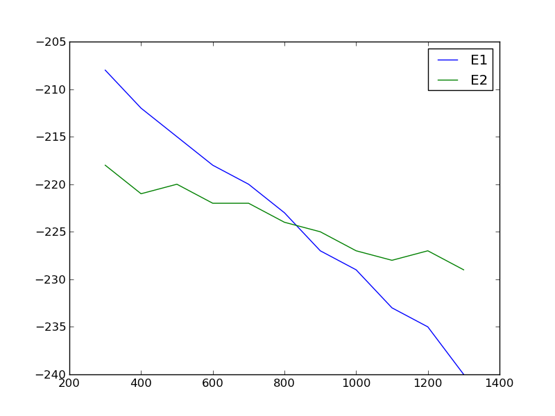
We want to determine the temperature at which they intersect, and more importantly what the uncertainty on the intersection is. There is noise in the data, which means there is uncertainty in any function that could be fit to it, and that uncertainty would propagate to the intersection. Let us examine the data.

import matplotlib.pyplot as plt

T = [x[0] for x in data]
E1 = [x[1] for x in data]
E2 = [x[2] for x in data]

plt.plot(T, E1, T, E2)
plt.legend(['E1', 'E2'])
plt.savefig('images/intersection-0.png')

Our strategy is going to be to fit functions to each data set, and get the confidence intervals on the parameters of the fit. Then, we will solve the equations to find where they are equal to each other and propagate the uncertainties in the parameters to the answer.

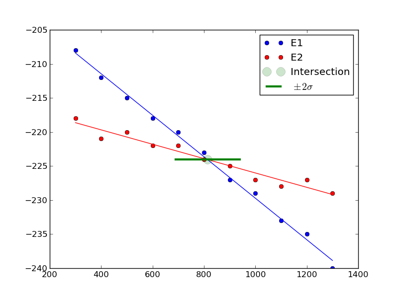
These functions look approximately linear, so we will fit lines to each function. We use the regress function in pycse to get the uncertainties on the fits. Then, we use the uncertainties package to propagate the uncertainties in the analytical solution to the intersection of two lines.

import numpy as np
from pycse import regress
import matplotlib.pyplot as plt
import uncertainties as u

T = np.array([x[0] for x in data])
E1 = np.array([x[1] for x in data])
E2 = np.array([x[2] for x in data])

# columns of the x-values for a line: constant, T
A = np.column_stack([T**0, T])

p1, pint1, se1 = regress(A, E1, alpha=0.05)

p2, pint2, se2 = regress(A, E2, alpha=0.05)

# Now we have two lines: y1 = m1*T + b1 and y2 = m2*T + b2
# they intersect at m1*T + b1 = m2*T + b2
# or at T = (b2 - b1) / (m1 - m2)
b1 = u.ufloat((p1[0], se1[0]))
m1 = u.ufloat((p1[1], se1[1]))

b2 = u.ufloat((p2[0], se2[0]))
m2 = u.ufloat((p2[1], se2[1]))

T_intersection = (b2 - b1) / (m1 - m2)
print T_intersection

# plot the data, the fits and the intersection and \pm 2 \sigma.
plt.plot(T, E1, 'bo ', label='E1')
plt.plot(T, np.dot(A,p1), 'b-')
plt.plot(T, E2, 'ro ', label='E2')
plt.plot(T, np.dot(A,p2), 'r-')

plt.plot(T_intersection.nominal_value,
        (b1 + m1*T_intersection).nominal_value, 'go',
        ms=13, alpha=0.2, label='Intersection')
plt.plot([T_intersection.nominal_value - 2*T_intersection.std_dev(),
          T_intersection.nominal_value + 2*T_intersection.std_dev()],
         [(b1 + m1*T_intersection).nominal_value, 
          (b1 + m1*T_intersection).nominal_value],
         'g-', lw=3, label='$\pm 2 \sigma$')
       
plt.legend(loc='best')
plt.savefig('images/intersection-1.png')
813.698630137+/-62.407180552

You can see there is a substantial uncertainty in the temperature at approximately the 90% confidence level (± 2 σ).

Update 7-7-2013

After a suggestion from Prateek, here we subtract the two data sets, fit a line to that data, and then use fsolve to find the zero. We wrap fsolve in the uncertainties package to directly get the uncertainty on the root.

import numpy as np
from pycse import regress
import matplotlib.pyplot as plt
import uncertainties as u
from scipy.optimize import fsolve


T = np.array([x[0] for x in data])
E1 = np.array([x[1] for x in data])
E2 = np.array([x[2] for x in data])

E = E1 - E2

# columns of the x-values for a line: constant, T
A = np.column_stack([T**0, T])

p, pint, se = regress(A, E, alpha=0.05)

b = u.ufloat((p[0], se[0]))
m = u.ufloat((p[1], se[1]))

@u.wrap
def f(b, m):
    X, = fsolve(lambda x: b + m * x, 800)
    return X

print f(b, m)
813.698630137+/-54.0386903923

Interesting that this uncertainty is a little smaller than the previously computed uncertainty. Here you can see we have to wrap the function in a peculiar way. The function must return a single float number, and take arguments with uncertainty. We define the polynomial fit (a line in this case) in a lambda function inside the function. It works ok.

Copyright (C) 2013 by John Kitchin. See the License for information about copying.

org-mode source
Discuss on Twitter

Constrained fits to data

| categories: data analysis, optimization | tags:

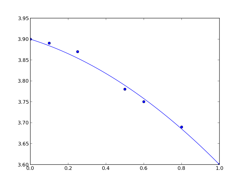
Our objective here is to fit a quadratic function in the least squares sense to some data, but we want to constrain the fit so that the function has specific values at the end-points. The application is to fit a function to the lattice constant of an alloy at different compositions. We constrain the fit because we know the lattice constant of the pure metals, which are at the end-points of the fit and we want these to be correct.

We define the alloy composition in terms of the mole fraction of one species, e.g. \(A_xB_{1-x}\). For \(x=0\), the alloy is pure B, whereas for \(x=1\) the alloy is pure A. According to Vegard's law the lattice constant is a linear composition weighted average of the pure component lattice constants, but sometimes small deviations are observed. Here we will fit a quadratic function that is constrained to give the pure metal component lattice constants at the end points.

The quadratic function is \(y = a x^2 + b x + c\). One constraint is at \(x=0\) where \(y = c\), or \(c\) is the lattice constant of pure B. The second constraint is at \(x=1\), where \(a + b + c\) is equal to the lattice constant of pure A. Thus, there is only one degree of freedom. \(c = LC_B\), and \(b = LC_A - c - a\), so \(a\) is our only variable.

We will solve this problem by minimizing the summed squared error between the fit and the data. We use the fmin function in scipy.optimize. First we create a fit function that encodes the constraints. Then we create an objective function that will be minimized. We have to make a guess about the value of \(a\) that minimizes the summed squared error. A line fits the data moderately well, so we guess a small value, i.e. near zero, for \(a\). Here is the solution.

import numpy as np
import matplotlib.pyplot as plt

# Data to fit to
# x=0 is pure B
# x=1 is pure A
X = np.array([0.0, 0.1,  0.25, 0.5,  0.6,  0.8,  1.0])
Y = np.array([3.9, 3.89, 3.87, 3.78, 3.75, 3.69, 3.6])

def func(a, XX):
    LC_A = 3.6
    LC_B = 3.9

    c = LC_B
    b = LC_A - c - a

    yfit = a * XX**2 + b * XX + c
    return yfit

def objective(a):
    'function to minimize'
    SSE = np.sum((Y - func(a, X))**2)
    return SSE


from scipy.optimize import fmin

a_fit = fmin(objective, 0)
plt.plot(X, Y, 'bo ')

x = np.linspace(0, 1)
plt.plot(x, func(a_fit, x))
plt.savefig('images/constrained-quadratic-fit.png')
Optimization terminated successfully.
         Current function value: 0.000445
         Iterations: 19
         Function evaluations: 38

Here is the result:

You can see that the end points go through the end-points as prescribed.

Copyright (C) 2013 by John Kitchin. See the License for information about copying.

org-mode source
Discuss on Twitter
Next Page ยป