Peak finding in Raman spectroscopy

| categories: data analysis | tags:

Table of Contents

Raman spectroscopy is a vibrational spectroscopy. The data typically comes as intensity vs. wavenumber, and it is discrete. Sometimes it is necessary to identify the precise location of a peak. In this post, we will use spline smoothing to construct an interpolating function of the data, and then use fminbnd to identify peak positions.

This example was originally worked out in Matlab at http://matlab.cheme.cmu.edu/2012/08/27/peak-finding-in-raman-spectroscopy/

numpy:loadtxt

Let us take a look at the raw data.

import numpy as np
import matplotlib.pyplot as plt

w, i = np.loadtxt('data/raman.txt', usecols=(0, 1), unpack=True)

plt.plot(w, i)
plt.xlabel('Raman shift (cm$^{-1}$)')
plt.ylabel('Intensity (counts)')
plt.savefig('images/raman-1.png')
plt.show()
>>> [<matplotlib.lines.Line2D object at 0x10b1d3190>]
<matplotlib.text.Text object at 0x10b1b1b10>
<matplotlib.text.Text object at 0x10bc7f310>

The next thing to do is narrow our focus to the region we are interested in between 1340 cm^{-1} and 1360 cm^{-1}.

ind = (w > 1340) & (w < 1360)
w1 = w[ind]
i1 = i[ind]

plt.plot(w1, i1, 'b. ')
plt.xlabel('Raman shift (cm$^{-1}$)')
plt.ylabel('Intensity (counts)')
plt.savefig('images/raman-2.png')
plt.show()
>>> >>> >>> [<matplotlib.lines.Line2D object at 0x10bc7a4d0>]
<matplotlib.text.Text object at 0x10bc08090>
<matplotlib.text.Text object at 0x10bc49710>

Next we consider a scipy:UnivariateSpline. This function "smooths" the data.

from scipy.interpolate import UnivariateSpline

# s is a "smoothing" factor
sp = UnivariateSpline(w1, i1, k=4, s=2000)

plt.plot(w1, i1, 'b. ')
plt.plot(w1, sp(w1), 'r-')
plt.xlabel('Raman shift (cm$^{-1}$)')
plt.ylabel('Intensity (counts)')
plt.savefig('images/raman-3.png')
plt.show()
>>> ... >>> >>> [<matplotlib.lines.Line2D object at 0x1105633d0>]
[<matplotlib.lines.Line2D object at 0x10dd70250>]
<matplotlib.text.Text object at 0x10dd65f10>
<matplotlib.text.Text object at 0x1105409d0>

Note that the UnivariateSpline function returns a "callable" function! Our next goal is to find the places where there are peaks. This is defined by the first derivative of the data being equal to zero. It is easy to get the first derivative of a UnivariateSpline with a second argument as shown below.

# get the first derivative evaluated at all the points
d1s = sp.derivative()

d1 = d1s(w1)

# we can get the roots directly here, which correspond to minima and
# maxima.
print('Roots = {}'.format(sp.derivative().roots()))
minmax = sp.derivative().roots()

plt.clf()
plt.plot(w1, d1, label='first derivative')
plt.xlabel('Raman shift (cm$^{-1}$)')
plt.ylabel('First derivative')
plt.grid()

plt.plot(minmax, d1s(minmax), 'ro ', label='zeros')
plt.legend(loc='best')

plt.plot(w1, i1, 'b. ')
plt.plot(w1, sp(w1), 'r-')
plt.xlabel('Raman shift (cm$^{-1}$)')
plt.ylabel('Intensity (counts)')
plt.plot(minmax, sp(minmax), 'ro ')

plt.savefig('images/raman-4.png')
>>> >>> >>> >>> ... ... Roots = [ 1346.4623087   1347.42700893  1348.16689639]
>>> >>> >>> [<matplotlib.lines.Line2D object at 0x1106b2dd0>]
<matplotlib.text.Text object at 0x110623910>
<matplotlib.text.Text object at 0x110c0a090>
>>> >>> [<matplotlib.lines.Line2D object at 0x10b1bacd0>]
<matplotlib.legend.Legend object at 0x1106b2650>
[<matplotlib.lines.Line2D object at 0x1106b2b50>]
[<matplotlib.lines.Line2D object at 0x110698550>]
<matplotlib.text.Text object at 0x110623910>
<matplotlib.text.Text object at 0x110c0a090>
[<matplotlib.lines.Line2D object at 0x110698a10>]

In the end, we have illustrated how to construct a spline smoothing interpolation function and to find maxima in the function, including generating some initial guesses. There is more art to this than you might like, since you have to judge how much smoothing is enough or too much. With too much, you may smooth peaks out. With too little, noise may be mistaken for peaks.

1 Summary notes

Using org-mode with :session allows a large script to be broken up into mini sections. However, it only seems to work with the default python mode in Emacs, and it does not work with emacs-for-python or the latest python-mode. I also do not really like the output style, e.g. the output from the plotting commands.

Copyright (C) 2014 by John Kitchin. See the License for information about copying.

org-mode source

Org-mode version = 8.2.7c

Discuss on Twitter

Graphical methods to help get initial guesses for multivariate nonlinear regression

| categories: plotting, data analysis | tags:

Matlab post

Fit the model f(x1,x2; a,b) = a*x1 + x2^b to the data given below. This model has two independent variables, and two parameters.

We want to do a nonlinear fit to find a and b that minimize the summed squared errors between the model predictions and the data. With only two variables, we can graph how the summed squared error varies with the parameters, which may help us get initial guesses. Let us assume the parameters lie in a range, here we choose 0 to 5. In other problems you would adjust this as needed.

import numpy as np
from mpl_toolkits.mplot3d import Axes3D
import matplotlib.pyplot as plt

x1 = [1.0, 2.0, 3.0, 4.0, 5.0, 6.0]
x2 = [0.2, 0.4, 0.8, 0.9, 1.1, 2.1]
X = np.column_stack([x1, x2]) # independent variables

f = [ 3.3079,    6.6358,   10.3143,   13.6492,   17.2755,   23.6271]

fig = plt.figure()
ax = fig.gca(projection = '3d')

ax.plot(x1, x2, f)
ax.set_xlabel('x1')
ax.set_ylabel('x2')
ax.set_zlabel('f(x1,x2)')

plt.savefig('images/graphical-mulvar-1.png')


arange = np.linspace(0,5);
brange = np.linspace(0,5);

A,B = np.meshgrid(arange, brange)

def model(X, a, b):
    'Nested function for the model'
    x1 = X[:, 0]
    x2 = X[:, 1]
    
    f = a * x1 + x2**b
    return f

@np.vectorize
def errfunc(a, b):
    # function for the summed squared error
    fit = model(X, a, b)
    sse = np.sum((fit - f)**2)
    return sse

SSE = errfunc(A, B)

plt.clf()
plt.contourf(A, B, SSE, 50)
plt.plot([3.2], [2.1], 'ro')
plt.figtext( 3.4, 2.2, 'Minimum near here', color='r')

plt.savefig('images/graphical-mulvar-2.png')

guesses = [3.18, 2.02]

from scipy.optimize import curve_fit

popt, pcov = curve_fit(model, X, f, guesses)
print popt

plt.plot([popt[0]], [popt[1]], 'r*')
plt.savefig('images/graphical-mulvar-3.png')

print model(X, *popt)

fig = plt.figure()
ax = fig.gca(projection = '3d')

ax.plot(x1, x2, f, 'ko', label='data')
ax.plot(x1, x2, model(X, *popt), 'r-', label='fit')
ax.set_xlabel('x1')
ax.set_ylabel('x2')
ax.set_zlabel('f(x1,x2)')

plt.savefig('images/graphical-mulvar-4.png')
[ 3.21694798  1.9728254 ]
[  3.25873623   6.59792994  10.29473657  13.68011436  17.29161001
  23.62366445]

It can be difficult to figure out initial guesses for nonlinear fitting problems. For one and two dimensional systems, graphical techniques may be useful to visualize how the summed squared error between the model and data depends on the parameters.

Copyright (C) 2013 by John Kitchin. See the License for information about copying.

org-mode source

Discuss on Twitter

Model selection

| categories: statistics, data analysis | tags:

Matlab post

adapted from http://www.itl.nist.gov/div898/handbook/pmd/section4/pmd44.htm

In this example, we show some ways to choose which of several models fit data the best. We have data for the total pressure and temperature of a fixed amount of a gas in a tank that was measured over the course of several days. We want to select a model that relates the pressure to the gas temperature.

The data is stored in a text file download PT.txt , with the following structure:

Run          Ambient                            Fitted
 Order  Day  Temperature  Temperature  Pressure    Value    Residual
  1      1      23.820      54.749      225.066   222.920     2.146
...

We need to read the data in, and perform a regression analysis on P vs. T. In python we start counting at 0, so we actually want columns 3 and 4.

import numpy as np
import matplotlib.pyplot as plt

data = np.loadtxt('data/PT.txt', skiprows=2)
T = data[:, 3]
P = data[:, 4]

plt.plot(T, P, 'k.')
plt.xlabel('Temperature')
plt.ylabel('Pressure')
plt.savefig('images/model-selection-1.png')
>>> >>> >>> >>> >>> >>> [<matplotlib.lines.Line2D object at 0x00000000084398D0>]
<matplotlib.text.Text object at 0x000000000841F6A0>
<matplotlib.text.Text object at 0x0000000008423DD8>

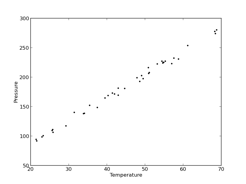
It appears the data is roughly linear, and we know from the ideal gas law that PV = nRT, or P = nR/V*T, which says P should be linearly correlated with V. Note that the temperature data is in degC, not in K, so it is not expected that P=0 at T = 0. We will use linear algebra to compute the line coefficients.

A = np.vstack([T**0, T]).T
b = P

x, res, rank, s = np.linalg.lstsq(A, b)
intercept, slope = x
print 'b, m =', intercept, slope

n = len(b)
k = len(x)

sigma2 = np.sum((b - np.dot(A,x))**2) / (n - k)

C = sigma2 * np.linalg.inv(np.dot(A.T, A))
se = np.sqrt(np.diag(C))

from scipy.stats.distributions import  t
alpha = 0.05

sT = t.ppf(1-alpha/2., n - k) # student T multiplier
CI = sT * se

print 'CI = ',CI
for beta, ci in zip(x, CI):
    print '[{0} {1}]'.format(beta - ci, beta + ci)
>>> >>> >>> >>> b, m = 7.74899739238 3.93014043824
>>> >>> >>> >>> >>> >>> >>> >>> >>> >>> >>> >>> >>> >>> >>> CI =  [ 4.76511545  0.1026405 ]
... ... [2.98388194638 12.5141128384]
[3.82749994079 4.03278093569]

The confidence interval on the intercept is large, but it does not contain zero at the 95% confidence level.

The R^2 value accounts roughly for the fraction of variation in the data that can be described by the model. Hence, a value close to one means nearly all the variations are described by the model, except for random variations.

ybar = np.mean(P)
SStot = np.sum((P - ybar)**2)
SSerr = np.sum((P - np.dot(A, x))**2)
R2 = 1 - SSerr/SStot
print R2
>>> >>> >>> 0.993715411798
plt.figure(); plt.clf()
plt.plot(T, P, 'k.', T, np.dot(A, x), 'b-')
plt.xlabel('Temperature')
plt.ylabel('Pressure')
plt.title('R^2 = {0:1.3f}'.format(R2))
plt.savefig('images/model-selection-2.png')
<matplotlib.figure.Figure object at 0x0000000008423860>
[<matplotlib.lines.Line2D object at 0x00000000085BE780>, <matplotlib.lines.Line2D object at 0x00000000085BE940>]
<matplotlib.text.Text object at 0x0000000008449898>
<matplotlib.text.Text object at 0x000000000844CCF8>
<matplotlib.text.Text object at 0x000000000844ED30>

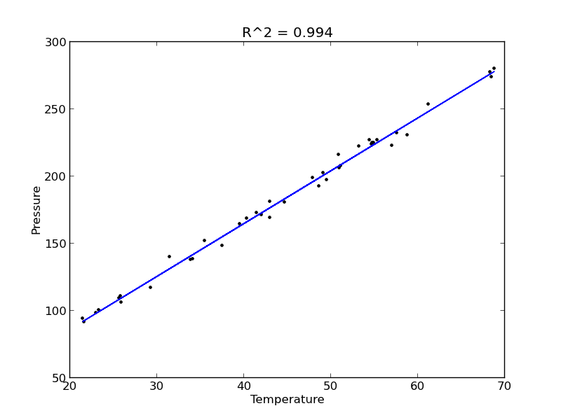
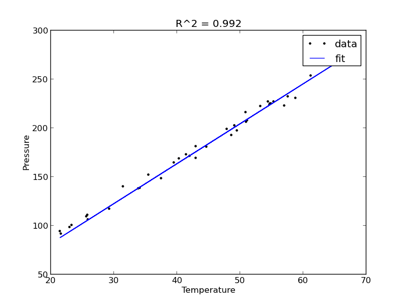
The fit looks good, and R^2 is near one, but is it a good model? There are a few ways to examine this. We want to make sure that there are no systematic trends in the errors between the fit and the data, and we want to make sure there are not hidden correlations with other variables. The residuals are the error between the fit and the data. The residuals should not show any patterns when plotted against any variables, and they do not in this case.

residuals = P - np.dot(A, x)

plt.figure()

f, (ax1, ax2, ax3) = plt.subplots(3)

ax1.plot(T,residuals,'ko')
ax1.set_xlabel('Temperature')


run_order = data[:, 0]
ax2.plot(run_order, residuals,'ko ')
ax2.set_xlabel('run order')

ambientT = data[:, 2]
ax3.plot(ambientT, residuals,'ko')
ax3.set_xlabel('ambient temperature')

plt.tight_layout() # make sure plots do not overlap

plt.savefig('images/model-selection-3.png')
>>> <matplotlib.figure.Figure object at 0x00000000085C21D0>
>>> >>> >>> [<matplotlib.lines.Line2D object at 0x0000000008861CC0>]
<matplotlib.text.Text object at 0x00000000085D3A58>
>>> >>> >>> [<matplotlib.lines.Line2D object at 0x0000000008861E80>]
<matplotlib.text.Text object at 0x00000000085EC5F8>
>>> >>> [<matplotlib.lines.Line2D object at 0x0000000008861C88>]
<matplotlib.text.Text object at 0x0000000008846828>

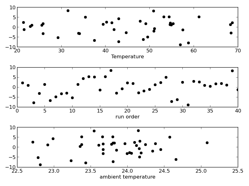
There may be some correlations in the residuals with the run order. That could indicate an experimental source of error.

We assume all the errors are uncorrelated with each other. We can use a lag plot to assess this, where we plot residual[i] vs residual[i-1], i.e. we look for correlations between adjacent residuals. This plot should look random, with no correlations if the model is good.

plt.figure(); plt.clf()
plt.plot(residuals[1:-1], residuals[0:-2],'ko')
plt.xlabel('residual[i]')
plt.ylabel('residual[i-1]')
plt.savefig('images/model-selection-correlated-residuals.png')
<matplotlib.figure.Figure object at 0x000000000886EB00>
[<matplotlib.lines.Line2D object at 0x0000000008A02908>]
<matplotlib.text.Text object at 0x00000000089E8198>
<matplotlib.text.Text object at 0x00000000089EB908>

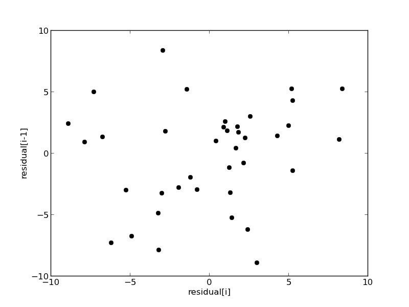
It is hard to argue there is any correlation here.

Lets consider a quadratic model instead.

A = np.vstack([T**0, T, T**2]).T
b = P;

x, res, rank, s = np.linalg.lstsq(A, b)
print x

n = len(b)
k = len(x)

sigma2 = np.sum((b - np.dot(A,x))**2) / (n - k)

C = sigma2 * np.linalg.inv(np.dot(A.T, A))
se = np.sqrt(np.diag(C))

from scipy.stats.distributions import  t
alpha = 0.05

sT = t.ppf(1-alpha/2., n - k) # student T multiplier
CI = sT * se

print 'CI = ',CI
for beta, ci in zip(x, CI):
    print '[{0} {1}]'.format(beta - ci, beta + ci)


ybar = np.mean(P)
SStot = np.sum((P - ybar)**2)
SSerr = np.sum((P - np.dot(A,x))**2)
R2 = 1 - SSerr/SStot
print 'R^2 = {0}'.format(R2)
>>> >>> >>> [  9.00353031e+00   3.86669879e+00   7.26244301e-04]
>>> >>> >>> >>> >>> >>> >>> >>> >>> >>> >>> >>> >>> >>> >>> CI =  [  1.38030344e+01   6.62100654e-01   7.48516727e-03]
... ... [-4.79950412123 22.8065647329]
[3.20459813681 4.52879944409]
[-0.00675892296907 0.00821141157035]
>>> >>> >>> >>> >>> R^2 = 0.993721969407

You can see that the confidence interval on the constant and T^2 term includes zero. That is a good indication this additional parameter is not significant. You can see also that the R^2 value is not better than the one from a linear fit, so adding a parameter does not increase the goodness of fit. This is an example of overfitting the data. Since the constant in this model is apparently not significant, let us consider the simplest model with a fixed intercept of zero.

Let us consider a model with intercept = 0, P = alpha*T.

A = np.vstack([T]).T
b = P;

x, res, rank, s = np.linalg.lstsq(A, b)

n = len(b)
k = len(x)

sigma2 = np.sum((b - np.dot(A,x))**2) / (n - k)

C = sigma2 * np.linalg.inv(np.dot(A.T, A))
se = np.sqrt(np.diag(C))

from scipy.stats.distributions import  t
alpha = 0.05

sT = t.ppf(1-alpha/2.0, n - k) # student T multiplier
CI = sT * se

for beta, ci in zip(x, CI):
    print '[{0} {1}]'.format(beta - ci, beta + ci)

plt.figure()
plt.plot(T, P, 'k. ', T, np.dot(A, x))
plt.xlabel('Temperature')
plt.ylabel('Pressure')
plt.legend(['data', 'fit'])

ybar = np.mean(P)
SStot = np.sum((P - ybar)**2)
SSerr = np.sum((P - np.dot(A,x))**2)
R2 = 1 - SSerr/SStot
plt.title('R^2 = {0:1.3f}'.format(R2))
plt.savefig('images/model-selection-no-intercept.png')
>>> >>> >>> >>> >>> >>> >>> >>> >>> >>> >>> >>> >>> >>> >>> >>> >>> >>> ... ... [4.05680124495 4.12308349899]
<matplotlib.figure.Figure object at 0x0000000008870BE0>
[<matplotlib.lines.Line2D object at 0x00000000089F4550>, <matplotlib.lines.Line2D object at 0x00000000089F4208>]
<matplotlib.text.Text object at 0x0000000008A13630>
<matplotlib.text.Text object at 0x0000000008A16DA0>
<matplotlib.legend.Legend object at 0x00000000089EFD30>
>>> >>> >>> >>> >>> <matplotlib.text.Text object at 0x000000000B26C0B8>

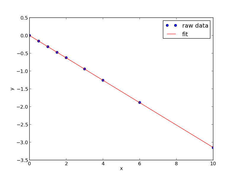
The fit is visually still pretty good, and the R^2 value is only slightly worse. Let us examine the residuals again.

residuals = P - np.dot(A,x)

plt.figure()
plt.plot(T,residuals,'ko')
plt.xlabel('Temperature')
plt.ylabel('residuals')
plt.savefig('images/model-selection-no-incpt-resid.png')
>>> <matplotlib.figure.Figure object at 0x0000000008A0F5C0>
[<matplotlib.lines.Line2D object at 0x000000000B29B0F0>]
<matplotlib.text.Text object at 0x000000000B276FD0>
<matplotlib.text.Text object at 0x000000000B283780>

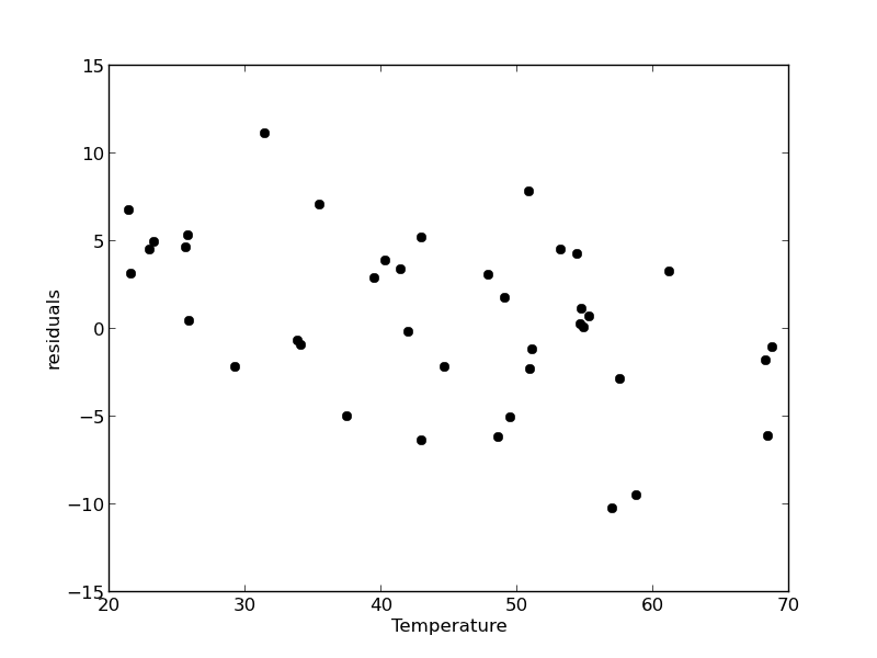
You can see a slight trend of decreasing value of the residuals as the Temperature increases. This may indicate a deficiency in the model with no intercept. For the ideal gas law in degC: \(PV = nR(T+273)\) or \(P = nR/V*T + 273*nR/V\), so the intercept is expected to be non-zero in this case. Specifically, we expect the intercept to be 273*R*n/V. Since the molar density of a gas is pretty small, the intercept may be close to, but not equal to zero. That is why the fit still looks ok, but is not as good as letting the intercept be a fitting parameter. That is an example of the deficiency in our model.

In the end, it is hard to justify a model more complex than a line in this case.

Copyright (C) 2013 by John Kitchin. See the License for information about copying.

org-mode source

Discuss on Twitter

Linear least squares fitting with linear algebra

| categories: linear algebra, data analysis | tags:

Matlab post

The idea here is to formulate a set of linear equations that is easy to solve. We can express the equations in terms of our unknown fitting parameters \(p_i\) as:

x1^0*p0 + x1*p1 = y1
x2^0*p0 + x2*p1 = y2
x3^0*p0 + x3*p1 = y3
etc...

Which we write in matrix form as \(A p = y\) where \(A\) is a matrix of column vectors, e.g. [1, x_i]. \(A\) is not a square matrix, so we cannot solve it as written. Instead, we form \(A^T A p = A^T y\) and solve that set of equations.

import numpy as np
x = np.array([0, 0.5, 1, 1.5, 2.0, 3.0, 4.0, 6.0, 10])
y = np.array([0, -0.157, -0.315, -0.472, -0.629, -0.942, -1.255, -1.884, -3.147])

A = np.column_stack([x**0, x])

M = np.dot(A.T, A)
b = np.dot(A.T, y)

i1, slope1 = np.dot(np.linalg.inv(M), b)
i2, slope2 = np.linalg.solve(M, b) # an alternative approach.

print i1, slope1
print i2, slope2

# plot data and fit
import matplotlib.pyplot as plt

plt.plot(x, y, 'bo')
plt.plot(x, np.dot(A, [i1, slope1]), 'r--')
plt.xlabel('x')
plt.ylabel('y')
plt.savefig('images/la-line-fit.png')
0.00062457337884 -0.3145221843
0.00062457337884 -0.3145221843

This method can be readily extended to fitting any polynomial model, or other linear model that is fit in a least squares sense. This method does not provide confidence intervals.

Copyright (C) 2013 by John Kitchin. See the License for information about copying.

org-mode source

Discuss on Twitter

Fit a line to numerical data

| categories: data analysis | tags:

Matlab post

We want to fit a line to this data:

x = [0, 0.5, 1, 1.5, 2.0, 3.0, 4.0, 6.0, 10]
y = [0, -0.157, -0.315, -0.472, -0.629, -0.942, -1.255, -1.884, -3.147]

We use the polyfit(x, y, n) command where n is the polynomial order, n=1 for a line.

import numpy as np

p = np.polyfit(x, y, 1)
print p
slope, intercept = p
print slope, intercept
>>> >>> [-0.31452218  0.00062457]
>>> -0.3145221843 0.00062457337884

To show the fit, we can use numpy.polyval to evaluate the fit at many points.

import matplotlib.pyplot as plt

xfit = np.linspace(0, 10)
yfit = np.polyval(p, xfit)

plt.plot(x, y, 'bo', label='raw data')
plt.plot(xfit, yfit, 'r-', label='fit')
plt.xlabel('x')
plt.ylabel('y')
plt.legend()
plt.savefig('images/linefit-1.png')
>>> >>> >>> >>> [<matplotlib.lines.Line2D object at 0x053C1790>]
[<matplotlib.lines.Line2D object at 0x0313C610>]
<matplotlib.text.Text object at 0x052A4950>
<matplotlib.text.Text object at 0x052B9A10>
<matplotlib.legend.Legend object at 0x053C1CD0>

Copyright (C) 2013 by John Kitchin. See the License for information about copying.

org-mode source

Discuss on Twitter
« Previous Page -- Next Page »