Solving Bessel's Equation numerically

| categories: ode, math | tags:

Matlab post

Reference Ch 5.5 Kreysig, Advanced Engineering Mathematics, 9th ed.

Bessel's equation \(x^2 y'' + x y' + (x^2 - \nu^2)y=0\) comes up often in engineering problems such as heat transfer. The solutions to this equation are the Bessel functions. To solve this equation numerically, we must convert it to a system of first order ODEs. This can be done by letting \(z = y'\) and \(z' = y''\) and performing the change of variables:

$$ y' = z$$

$$ z' = \frac{1}{x^2}(-x z - (x^2 - \nu^2) y$$

if we take the case where \(\nu = 0\), the solution is known to be the Bessel function \(J_0(x)\), which is represented in Matlab as besselj(0,x). The initial conditions for this problem are: \(y(0) = 1\) and \(y'(0)=0\).

There is a problem with our system of ODEs at x=0. Because of the \(1/x^2\) term, the ODEs are not defined at x=0. If we start very close to zero instead, we avoid the problem.

import numpy as np
from scipy.integrate import odeint
from scipy.special import jn # bessel function
import matplotlib.pyplot as plt

def fbessel(Y, x):
    nu = 0.0
    y = Y[0]
    z = Y[1]
  
    dydx = z
    dzdx = 1.0 / x**2 * (-x * z - (x**2 - nu**2) * y)
    return [dydx, dzdx]

x0 = 1e-15
y0 = 1
z0 = 0
Y0 = [y0, z0]

xspan = np.linspace(1e-15, 10)
sol = odeint(fbessel, Y0, xspan)

plt.plot(xspan, sol[:,0], label='numerical soln')
plt.plot(xspan, jn(0, xspan), 'r--', label='Bessel')
plt.legend()
plt.savefig('images/bessel.png')

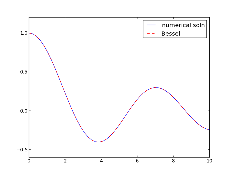
You can see the numerical and analytical solutions overlap, indicating they are at least visually the same.

Copyright (C) 2013 by John Kitchin. See the License for information about copying.

org-mode source

Discuss on Twitter

Solving parameterized ODEs over and over conveniently

| categories: ode | tags: reaction engineering

Matlab post Sometimes we have an ODE that depends on a parameter, and we want to solve the ODE for several parameter values. It is inconvenient to write an ode function for each parameter case. Here we examine a convenient way to solve this problem; we pass the parameter to the ODE at runtime. We consider the following ODE:

$$\frac{dCa}{dt} = -k Ca(t)$$

where \(k\) is a parameter, and we want to solve the equation for a couple of values of \(k\) to test the sensitivity of the solution on the parameter. Our question is, given \(Ca(t=0)=2\), how long does it take to get \(Ca = 1\), and how sensitive is the answer to small variations in \(k\)?

import numpy as np
from scipy.integrate import odeint
import matplotlib.pyplot as plt

def myode(Ca, t, k):
    'ODE definition'
    dCadt = -k * Ca
    return dCadt

tspan = np.linspace(0, 0.5)
k0 = 2
Ca0 = 2

plt.figure(); plt.clf()

for k in [0.95 * k0, k0, 1.05 * k0]:
    sol = odeint(myode, Ca0, tspan, args=(k,))
    plt.plot(tspan, sol, label='k={0:1.2f}'.format(k))
    print 'At t=0.5 Ca = {0:1.2f} mol/L'.format(sol[-1][0])

plt.legend(loc='best')
plt.xlabel('Time')
plt.ylabel('$C_A$ (mol/L)')
plt.savefig('images/parameterized-ode1.png')
At t=0.5 Ca = 0.77 mol/L
At t=0.5 Ca = 0.74 mol/L
At t=0.5 Ca = 0.70 mol/L

You can see there are some variations in the concentration at t = 0.5. You could over or underestimate the concentration if you have the wrong estimate of $k$! You have to use some judgement here to decide how long to run the reaction to ensure a target goal is met.

Copyright (C) 2013 by John Kitchin. See the License for information about copying.

org-mode source

Discuss on Twitter

Plotting ODE solutions in cylindrical coordinates

| categories: ode | tags:

Matlab post

It is straightforward to plot functions in Cartesian coordinates. It is less convenient to plot them in cylindrical coordinates. Here we solve an ODE in cylindrical coordinates, and then convert the solution to Cartesian coordinates for simple plotting.

import numpy as np
from scipy.integrate import odeint

def dfdt(F, t):
    rho, theta, z = F
    drhodt = 0   # constant radius
    dthetadt = 1 # constant angular velocity
    dzdt = -1    # constant dropping velocity
    return [drhodt, dthetadt, dzdt]

# initial conditions
rho0 = 1
theta0 = 0
z0 = 100

tspan = np.linspace(0, 50, 500)
sol = odeint(dfdt, [rho0, theta0, z0], tspan)

rho = sol[:,0]
theta = sol[:,1]
z = sol[:,2]

# convert cylindrical coords to cartesian for plotting.
X = rho * np.cos(theta)
Y = rho * np.sin(theta)

from mpl_toolkits.mplot3d import Axes3D
import matplotlib.pyplot as plt
fig = plt.figure()
ax = fig.gca(projection='3d')
ax.plot(X, Y, z)
plt.savefig('images/ode-cylindrical.png')

Copyright (C) 2013 by John Kitchin. See the License for information about copying.

org-mode source

Discuss on Twitter

Time dependent concentration in a first order reversible reaction in a batch reactor

| categories: ode | tags: reaction engineering

Matlab post

Given this reaction \(A \rightleftharpoons B\), with these rate laws:

forward rate law: \(-r_a = k_1 C_A\)

backward rate law: \(-r_b = k_{-1} C_B\)

plot the concentration of A vs. time. This example illustrates a set of coupled first order ODES.

from scipy.integrate import odeint
import numpy as np

def myode(C, t):
    # ra = -k1*Ca
    # rb = -k_1*Cb
    # net rate for production of A:  ra - rb
    # net rate for production of B: -ra + rb

    k1 = 1   # 1/min;
    k_1 = 0.5   # 1/min;

    Ca = C[0]
    Cb = C[1]

    ra = -k1 * Ca
    rb = -k_1 * Cb

    dCadt =  ra - rb
    dCbdt = -ra + rb

    dCdt = [dCadt, dCbdt]
    return dCdt

tspan = np.linspace(0, 5)

init = [1, 0]  # mol/L
C = odeint(myode, init, tspan)

Ca = C[:,0]
Cb = C[:,1]

import matplotlib.pyplot as plt
plt.plot(tspan, Ca, tspan, Cb)
plt.xlabel('Time (min)')
plt.ylabel('C (mol/L)')
plt.legend(['$C_A$', '$C_B$'])
plt.savefig('images/reversible-batch.png')

That is it. The main difference between this and Matlab is the order of arguments in odeint is different, and the ode function has differently ordered arguments.

Copyright (C) 2013 by John Kitchin. See the License for information about copying.

org-mode source

Discuss on Twitter

Solving a second order ode

| categories: ode, math | tags:

Matlab post

The odesolvers in scipy can only solve first order ODEs, or systems of first order ODES. To solve a second order ODE, we must convert it by changes of variables to a system of first order ODES. We consider the Van der Pol oscillator here:

$$\frac{d^2x}{dt^2} - \mu(1-x^2)\frac{dx}{dt} + x = 0$$

\(\mu\) is a constant. If we let \(y=x - x^3/3\) http://en.wikipedia.org/wiki/Van_der_Pol_oscillator, then we arrive at this set of equations:

$$\frac{dx}{dt} = \mu(x-1/3x^3-y)$$

$$\frac{dy}{dt} = \mu/x$$

here is how we solve this set of equations. Let \(\mu=1\).

from scipy.integrate import odeint
import numpy as np

mu = 1.0

def vanderpol(X, t):
    x = X[0]
    y = X[1]
    dxdt = mu * (x - 1./3.*x**3 - y)
    dydt = x / mu
    return [dxdt, dydt]

X0 = [1, 2]
t = np.linspace(0, 40, 250)

sol = odeint(vanderpol, X0, t)

import matplotlib.pyplot as plt
x = sol[:, 0]
y = sol[:, 1]

plt.plot(t,x, t, y)
plt.xlabel('t')
plt.legend(('x', 'y'))
plt.savefig('images/vanderpol-1.png')

# phase portrait
plt.figure()
plt.plot(x,y)
plt.plot(x[0], y[0], 'ro')
plt.xlabel('x')
plt.ylabel('y')
plt.savefig('images/vanderpol-2.png')

Here is the phase portrait. You can see that a limit cycle is approached, indicating periodicity in the solution.

Copyright (C) 2013 by John Kitchin. See the License for information about copying.

org-mode source

Discuss on Twitter
« Previous Page -- Next Page »