Solving differential algebraic equations with help from autograd

| categories: autograd, dae, ode | tags:

This problem is adapted from one in "Problem Solving in Chemical Engineering with Numerical Methods, Michael B. Cutlip, Mordechai Shacham".

In the binary, batch distillation of benzene (1) and toluene (2), the moles of liquid \(L\) remaining as a function of the mole fraction of toluene (\(x_2\)) is expressed by:

\(\frac{dL}{dx_2} = \frac{L}{x_2 (k_2 - 1)}\)

where \(k_2\) is the vapor liquid equilibrium ratio for toluene. This can be computed as:

\(k_i = P_i / P\) where \(P_i = 10^{A_i + \frac{B_i}{T +C_i}}\) and that pressure is in mmHg, and the temperature is in degrees Celsius.

One difficulty in solving this problem is that the temperature is not constant; it changes with the composition. We know that the temperature changes to satisfy this constraint \(k_1(T) x_1 + k_2(T) x_2 = 1\).

Sometimes, one can solve for T directly, and substitute it into the first ODE, but this is not a possibility here. One way you might solve this is to use the constraint to find \(T\) inside an ODE function, but that is tricky; nonlinear algebra solvers need a guess and don't always converge, or may converge to non-physical solutions. They also require iterative solutions, so they will be slower than an approach where we just have to integrate the solution. A better way is to derive a second ODE \(dT/dx_2\) from the constraint. The constraint is implicit in \(T\), so We compute it as \(dT/dx_2 = -df/dx_2 / df/dT\) where \(f(x_2, T) = k_1(T) x_1 + k_2(T) x_2 - 1 = 0\). This equation is used to compute the bubble point temperature. Note, it is possible to derive these analytically, but who wants to? We can use autograd to get those derivatives for us instead.

The following information is given:

The total pressure is fixed at 1.2 atm, and the distillation starts at \(x_2=0.4\). There are initially 100 moles in the distillation.

species A B C
benzene 6.90565 -1211.033 220.79
toluene 6.95464 -1344.8 219.482

We have to start by finding the initial temperature from the constraint.

import autograd.numpy as np
from autograd import grad
from scipy.integrate import solve_ivp
from scipy.optimize import fsolve
%matplotlib inline
import matplotlib.pyplot as plt

P = 760 * 1.2 # mmHg
A1, B1, C1 = 6.90565, -1211.033,  220.79
A2, B2, C2 = 6.95464, -1344.8, 219.482

def k1(T):
    return 10**(A1 + B1 / (C1 + T)) / P

def k2(T):
    return 10**(A2 + B2 / (C2 + T)) / P

def f(x2, T):
    x1 = 1 - x2
    return k1(T) * x1 + k2(T) * x2 - 1

T0, = fsolve(lambda T: f(0.4, T), 96)
print(f'The initial temperature is {T0:1.2f} degC.')

The initial temperature is 95.59 degC.

Next, we compute the derivative we need. This derivative is derived from the constraint, which should ensure that the temperature changes as required to maintain the constraint.

dfdx2 = grad(f, 0)
dfdT = grad(f, 1)

def dTdx2(x2, T):
    return -dfdx2(x2, T) / dfdT(x2, T)

def ode(x2, X):
    L, T = X
    dLdx2 = L / (x2 * (k2(T) - 1))
    return [dLdx2, dTdx2(x2, T)]

Next we solve and plot the ODE.

x2span = (0.4, 0.8)
X0 = (100, T0)
sol = solve_ivp(ode, x2span, X0, max_step=0.01)

plt.plot(sol.t, sol.y.T)
plt.legend(['L', 'T']);
plt.xlabel('$x_2$')
plt.ylabel('L, T')
x2 = sol.t
L, T = sol.y
print(f'At x2={x2[-1]:1.2f} there are {L[-1]:1.2f} moles of liquid left at {T[-1]:1.2f} degC')

At x2=0.80 there are 14.04 moles of liquid left at 108.57 degC

<Figure size 432x288 with 1 Axes>

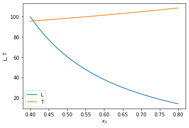
You can see that the liquid level drops, and the temperature rises.

Let's double check that the constraint is actually met. We do that qualitatively here by plotting it, and quantitatively by showing all values are close to 0.

constraint = k1(T) * (1 - x2) + k2(T) * x2 - 1
plt.plot(x2, constraint)
plt.ylim([-1, 1])
plt.xlabel('$x_2$')
plt.ylabel('constraint value')
print(np.allclose(constraint, np.zeros_like(constraint)))
constraint

True

array([ 2.22044605e-16,  4.44089210e-16,  2.22044605e-16,  0.00000000e+00,
        1.11022302e-15,  0.00000000e+00,  6.66133815e-16,  0.00000000e+00,
       -2.22044605e-16,  1.33226763e-15,  8.88178420e-16, -4.44089210e-16,
        4.44089210e-16,  1.11022302e-15, -2.22044605e-16,  0.00000000e+00,
       -2.22044605e-16, -1.11022302e-15,  4.44089210e-16,  0.00000000e+00,
       -4.44089210e-16,  4.44089210e-16, -6.66133815e-16, -4.44089210e-16,
        4.44089210e-16, -1.11022302e-16, -8.88178420e-16, -8.88178420e-16,
       -9.99200722e-16, -3.33066907e-16, -7.77156117e-16, -2.22044605e-16,
       -9.99200722e-16, -1.11022302e-15, -3.33066907e-16, -1.99840144e-15,
       -1.33226763e-15, -2.44249065e-15, -1.55431223e-15, -6.66133815e-16,
       -2.22044605e-16])
<Figure size 432x288 with 1 Axes>

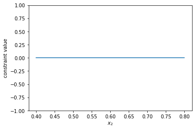
So indeed, the constraint is met! Once again, autograd comes to the rescue in making a computable derivative from an algebraic constraint so that we can solve a DAE as a set of ODEs using our regular machinery. Nice work autograd!

Copyright (C) 2019 by John Kitchin. See the License for information about copying.

org-mode source

Org-mode version = 9.2.3

Discuss on Twitter

Sensitivity analysis with odeint and autograd

| categories: autograd, ode | tags:

In this previous post I showed a way to do sensitivity analysis of the solution of a differential equation to parameters in the equation using autograd. The basic approach was to write a differentiable integrator, and then use it in a function so that autograd could take the derivative.

Since that time, autograd has added derivative support for scipy.integrate.odeint. In this post we examine that. As usual with autograd, we have to import the autograd version of numpy, and the autograd version of odeint. We will find the derivative of the solution to an ODE (which is an array) so we need to also import the jacobian function. Finally, there is a subtle, and non-obvious requirement that we need to import the autograd tuple. That ensures that the variables are differentiable through the tuple we will use for the arguments.

The differential equation we solve returns the concentration of a species as a function of time, and the solution depends on two parameters, i.e. \(C = f(t; k_1, k_{-1})\), and we are interested in the time-dependent sensitivity of \(C\) with respect to those parameters. The approach we use is to define a function that has those parameters as arguments. The function will solve the ODE and return the time-dependent solution. First we make that solution, mostly to see that the autograd version of odeint works.

import autograd.numpy as np
from autograd.scipy.integrate import odeint
from autograd import jacobian
from autograd.builtins import tuple

import matplotlib.pyplot as plt

Ca0 = 1.0
k1 = k_1 = 3.0

tspan = np.linspace(0, 0.5)

def C(K):
    k1, k_1 = K
    def dCdt(Ca, t, k1, k_1):
        return -k1 * Ca + k_1 * (Ca0 - Ca)
    sol = odeint(dCdt, Ca0, tspan, tuple((k1, k_1)))
    return sol

plt.plot(tspan, C([k1, k_1]))
plt.xlim([tspan.min(), tspan.max()])
plt.xlabel('t')
plt.ylabel('C');
<Figure size 432x288 with 1 Axes>

Now, the solution is an array, and we want the derivative of C with respect to the parameters at each time point. That means we want the jacobian derivative of the output with respect to the input. Here is the autograd approach to doing that. The jacobian function returns a function that we can evaluate to get the derivatives.

import time
t0 = time.time()
dCdk = jacobian(C, 0)


k_sensitivity = dCdk(np.array([k1, k_1]))

k1_sensitivity = k_sensitivity[:, 0, 0]
k_1_sensitivity = k_sensitivity[:, 0, 1]

plt.plot(tspan, np.abs(k1_sensitivity), label='dC/dk1')
plt.plot(tspan, np.abs(k_1_sensitivity), label='dC/dk_1')
plt.legend(loc='best')
plt.xlabel('t')
plt.ylabel('sensitivity')
print(f'Elapsed time = {time.time() - t0:1.1f} seconds')

Elapsed time = 38.2 seconds

<Figure size 432x288 with 1 Axes>

That looks similar to the results from before. It is pretty slow I think, that took more than half a minute to work out. That is still faster and probably more correct than if I had to do it by hand. In contrast, however, the finite difference code below is comparatively very fast! I don't know what is slow in the autograd implementation. I guess it is an implementation detail.

import numdifftools as nd
t0 = time.time()

fdk1, fdk_1 = nd.Jacobian(C)([k1, k_1]).T
print(f'Elapsed time = {time.time() - t0:1.1f} seconds')

plt.plot(tspan, np.abs(fdk1), label='fd dC/dk1')
plt.plot(tspan, np.abs(fdk_1), label='fd dC/dk_1')
plt.plot(tspan, np.abs(k1_sensitivity), 'y--', label='dC/dk1')
plt.plot(tspan, np.abs(k_1_sensitivity),'m--', label='dC/dk_1')
plt.legend(loc='best');
plt.xlabel('t');
plt.ylabel('sensitivity');

Elapsed time = 0.1 seconds

<Figure size 432x288 with 1 Axes>

You can see the two results are visually indistinguishable. Even the code is pretty similar. I would tend to prefer the autograd way since it should be less sensitive to finite difference artifacts, but it is nice to have an independent way to test if it is working.

Copyright (C) 2019 by John Kitchin. See the License for information about copying.

org-mode source

Org-mode version = 9.2.3

Discuss on Twitter

Solving coupled ODEs with a neural network and autograd

| categories: autograd, ode | tags:

In a previous post I wrote about using ideas from machine learning to solve an ordinary differential equation using a neural network for the solution. A friend recently tried to apply that idea to coupled ordinary differential equations, without success. It seems like that should work, so here we diagnose the issue and figure it out. This is a long post, but it works in the end.

In the classic series reaction \(A \rightarrow B \rightarrow C\) in a batch reactor, we get the set of coupled mole balances:

\(dC_A/dt = -k_1 C_A\)

\(dC_B/dt = k_1 C_A - k_2 C_B\)

\(dC_C/dt = k2 C_B\)

1 The standard numerical solution

Here is the standard numerical solution to this problem. This will give us a reference for what the solution should look like.

from scipy.integrate import solve_ivp

def ode(t, C):
    Ca, Cb, Cc = C
    dCadt = -k1 * Ca
    dCbdt = k1 * Ca - k2 * Cb
    dCcdt = k2 * Cb
    return [dCadt, dCbdt, dCcdt]

C0 = [1.0, 0.0, 0.0]
k1 = 1
k2 = 1

sol = solve_ivp(ode, (0, 10), C0)

%matplotlib inline
import matplotlib.pyplot as plt

plt.plot(sol.t, sol.y.T)
plt.legend(['A', 'B', 'C'])
plt.xlabel('Time')
plt.ylabel('C')

2 Can a neural network learn the solution?

The first thing I want to show is that you can train a neural network to reproduce this solution. That is certainly a prerequisite to the idea working. We use the same code I used before, but this time our neural network will output three values, one for each concentration.

import autograd.numpy as np
from autograd import grad, elementwise_grad, jacobian
import autograd.numpy.random as npr
from autograd.misc.optimizers import adam

def init_random_params(scale, layer_sizes, rs=npr.RandomState(0)):
    """Build a list of (weights, biases) tuples, one for each layer."""
    return [(rs.randn(insize, outsize) * scale,   # weight matrix
             rs.randn(outsize) * scale)           # bias vector
            for insize, outsize in zip(layer_sizes[:-1], layer_sizes[1:])]

def swish(x):
    "see https://arxiv.org/pdf/1710.05941.pdf"
    return x / (1.0 + np.exp(-x))

def C(params, inputs):
    "Neural network functions"
    for W, b in params:
        outputs = np.dot(inputs, W) + b
        inputs = swish(outputs)
    return outputs

# initial guess for the weights and biases
params = init_random_params(0.1, layer_sizes=[1, 8, 3])

Now, we train our network to reproduce the solution. I ran this block manually a bunch of times, but eventually you see that we can train a one layer network with 8 nodes to output all three concentrations pretty accurately. So, there is no issue there, a neural network can represent the solution.

def objective_soln(params, step):
    return np.sum((sol.y.T - C(params, sol.t.reshape([-1, 1])))**2)

params = adam(grad(objective_soln), params,
              step_size=0.001, num_iters=500)

plt.plot(sol.t.reshape([-1, 1]), C(params, sol.t.reshape([-1, 1])),
         sol.t, sol.y.T, 'o')
plt.legend(['A', 'B', 'C', 'Ann', 'Bnn', 'Cnn'])
plt.xlabel('Time')
plt.ylabel('C')

3 Given a neural network function how do we get the right derivatives?

The next issue is how do we get the relevant derivatives. The solution method I developed here relies on using optimization to find a set of weights that produces a neural network whose derivatives are consistent with the ODE equations. So, we need to be able to get the derivatives that are relevant in the equations.

The neural network outputs three concentrations, and we need the time derivatives of them. Autograd provides three options: grad, elementwise_grad and jacobian. We cannot use grad because our function is not scalar. We cannot use elementwise_grad because that will give the wrong shape (I think it may be the sum of the gradients). That leaves us with the jacobian. This, however, gives an initially unintuitive (i.e. it isn't what we need out of the box) result. The output is 4-dimensional in this case, consistent with the documentation of that function.

jacC = jacobian(C, 1)
jacC(params, sol.t.reshape([-1, 1])).shape
(17, 3, 17, 1)

Why does it have this shape? Our time input vector we used has 17 time values, in a column vector. That leads to an output from the NN with a shape of (17, 3), i.e. the concentrations of each species at each time. The jacobian will output an array of shape (17, 3, 17, 1), and we have to extract the pieces we want from that. The first and third dimensions are related to the time steps. The second dimension is the species, and the last dimension is nothing here, but is there because the input is in a column. I use some fancy indexing on the array to get the desired arrays of the derivatives. This is not obvious out of the box. I only figured this out by direct comparison of the data from a numerical solution and the output of the jacobian. Here I show how to do that, and make sure that the derivatives we pull out are comparable to the derivatives defined by the ODEs above. Parity here means they are comparable.

i = np.arange(len(sol.t))
plt.plot(jacC(params, sol.t.reshape([-1, 1]))[i, 0, i, 0],   -k1 * sol.y[0], 'ro')
plt.plot(jacC(params, sol.t.reshape([-1, 1]))[i, 1, i, 0],   -k2 * sol.y[1] + k1 * sol.y[0], 'bo')
plt.plot(jacC(params, sol.t.reshape([-1, 1]))[i, 2, i, 0],   k2 * sol.y[1], 'go')
[<matplotlib.lines.Line2D at 0x118a2e860>]

Note this is pretty inefficient. It requires a lot of calculations (the jacobian here has print(17*3*17) 867 elements) to create the jacobian, and we don't need most of them. You could avoid this by creating separate neural networks for each species, and then just use elementwise_grad on each one. Alternatively, one might be able to more efficiently compute some vector-jacobian product. Nevertheless, it looks like we can get the correct derivatives out of the neural network, we just need a convenient function to return them. Here is one such function for this problem, using a fancier slicing and reshaping to get the derivative array.

# Derivatives
jac = jacobian(C, 1)

def dCdt(params, t):
    i = np.arange(len(t))
    return jac(params, t)[i, :, i].reshape((len(t), 3))

4 Solving the system of ODEs with a neural network

Finally, we are ready to try solving the ODEs solely by the neural network approach. We reinitialize the neural network first, and define a time grid to solve it on.

t = np.linspace(0, 10, 25).reshape((-1, 1))
params = init_random_params(0.1, layer_sizes=[1, 8, 3])
i = 0    # number of training steps
N = 501  # epochs for training
et = 0.0 # total elapsed time

We define our objective function. This function will be zero at the perfect solution, and has contributions for each mole balance and the initial conditions. It could make sense to put additional penalties for things like negative concentrations, or the sum of concentrations is a constant, but we do not do that here, and it does not seem to be necessary.

def objective(params, step):
    Ca, Cb, Cc = C(params, t).T
    dCadt, dCbdt, dCcdt = dCdt(params, t).T

    z1 = np.sum((dCadt + k1 * Ca)**2)
    z2 = np.sum((dCbdt - k1 * Ca + k2 * Cb)**2)
    z3 = np.sum((dCcdt - k2 * Cb)**2)
    ic = np.sum((np.array([Ca[0], Cb[0], Cc[0]]) - C0)**2)  # initial conditions
    return z1 + z2 + z3 + ic

def callback(params, step, g):
    if step % 100 == 0:
        print("Iteration {0:3d} objective {1}".format(step,
                                                      objective(params, step)))

objective(params, 0)  # make sure the objective is scalar
5.2502237371050295

Finally, we run the optimization. I also manually ran this block several times.

import time
t0 = time.time()

params = adam(grad(objective), params,
              step_size=0.001, num_iters=N, callback=callback)

i += N
t1 = (time.time() - t0) / 60
et += t1

plt.plot(t, C(params, t), sol.t, sol.y.T, 'o')
plt.legend(['Ann', 'Bnn', 'Cnn', 'A', 'B', 'C'])
plt.xlabel('Time')
plt.ylabel('C')
print(f'{t1:1.1f} minutes elapsed this time. Total time = {et:1.2f} min. Total epochs = {i}.')
Iteration   0 objective 0.00047651643957525214
Iteration 100 objective 0.0004473301532609342
Iteration 200 objective 0.00041218410058863227
Iteration 300 objective 0.00037161526137030344
Iteration 400 objective 0.000327567400443358
Iteration 500 objective 0.0002836975879675981
0.6 minutes elapsed this time. Total time = 4.05 min. Total epochs = 3006.


The effort seems to have been worth it though, we get a pretty good solution from our neural network.

We can check the accuracy of the derivatives by noting the sum of the derivatives in this case should be zero. Here you can see that the sum is pretty small. It would take additional optimization to a lower error to get this to be smaller.

plt.plot(t, np.sum(dCdt(params, t), axis=1))
plt.xlabel('Time')
plt.ylabel(r'$\Sigma dC/dt$')

5 Summary

In the end, this method is illustrated to work for systems of ODEs also. There is some subtlety in how to get the relevant derivatives from the jacobian, but after that, it is essentially the same. I think it would be much faster to do this with separate neural networks for each function in the solution because then you do not need the jacobian, you can use elementwise_grad.

This is not faster than direct numerical integration. One benefit to this solution over a numerical solution is we get an actual continuous function as the solution, rather than an array of data. This solution is not reliable at longer times, but then again neither is extrapolation of numeric data. It could be interesting to explore if this has any benefits for stiff equations. Maybe another day. For now, I am declaring victory for autograd on this problem.

Copyright (C) 2018 by John Kitchin. See the License for information about copying.

org-mode source

Org-mode version = 9.1.14

Discuss on Twitter

A differentiable ODE integrator for sensitivity analysis

| categories: sensitivity, autograd, ode | tags:

Last time I wrote about using automatic differentiation to find the derivative of an integral function. A related topic is finding derivatives of functions that are defined by differential equations. We typically use a numerical integrator to find solutions to these functions. Those leave us with numeric solutions which we then have to use to approximate derivatives. What if the integrator itself was differentiable? It is after all, just a program, and automatic differentiation should be able to tell us the derivatives of functions that use them. This is not a new idea, there is already a differentiable ODE solver in Tensorflow. Here I will implement a simple Runge Kutta integrator and then show how we can use automatic differentiation to do sensitivity analysis on the numeric solution.

I previously used autograd for sensitivity analysis on analytical solutions in this post. Here I will compare those results to the results from sensitivity analysis on the numerical solutions.

First, we need an autograd compatible ODE integrator. Here is one implementation of a simple, fourth order Runge-Kutta integrator. Usually, I would use indexing to do this, but that was not compatible with autograd, so I just accumulate the solution. This is a limitation of autograd, and it is probably not an issue with Tensorflow, for example, or probably pytorch. Those are more sophisticated, and more difficult to use packages than autograd. Here I am just prototyping an idea, so we stick with autograd.

import autograd.numpy as np
from autograd import grad
%matplotlib inline
import matplotlib.pyplot as plt

def rk4(f, tspan, y0, N=50):
    x, h = np.linspace(*tspan, N, retstep=True)
    y = []
    y = y + [y0]
    for i in range(0, len(x) - 1):
        k1 = h * f(x[i], y[i])
        k2 = h * f(x[i] + h / 2, y[i] + k1 / 2)
        k3 = h * f(x[i] + h / 2, y[i] + k2 / 2)
        k4 = h * f(x[i + 1], y[i] + k3)
        y += [y[-1] + (k1 + (2 * k2) + (2 * k3) + k4) / 6]
    return x, y

Now, we just check that it works as expected:

Ca0 = 1.0
k1 = k_1 = 3.0

def dCdt(t, Ca):
    return -k1 * Ca + k_1 * (Ca0 - Ca)

t, Ca = rk4(dCdt, (0, 0.5), Ca0)

def analytical_A(t, k1, k_1):
    return Ca0 / (k1 + k_1) * (k1 * np.exp(-(k1 + k_1) * t) + k_1)

plt.plot(t, Ca, label='RK4')
plt.plot(t, analytical_A(t, k1, k_1), 'r--', label='analytical')
plt.xlabel('t')
plt.ylabel('[A]')
plt.xlim([0, 0.5])
plt.ylim([0.5, 1])
plt.legend()

That looks fine, we cannot visually distinguish the two solutions, and they both look like Figure 1 in this paper. Note the analytical solution is not that complex, but it would not take much variation of the rate law to make this solution difficult to derive.

Next, to do sensitivity analysis, we need to define a function for \(A\) that depends on the rate constants, so we can take a derivative of it with respect to the parameters we want the sensitivity from. We seek the derivatives: \(\frac{dC_A}{dk_1}\) and \(\frac{dC_A}{dk_{-1}}\). Here is a function that does that. It will return the value of [A] at \(t\) given an initial concentration and the rate constants.

def A(Ca0, k1, k_1, t):
    def dCdt(t, Ca):
        return -k1 * Ca + k_1 * (Ca0 - Ca)
    t, Ca_ = rk4(dCdt, (0, t), Ca0)
    return Ca_[-1]

# Here are the two derivatives we seek.
dCadk1 = grad(A, 1)
dCadk_1 = grad(A, 2)

We also use autograd to get the derivatives from the analytical solution for comparison.

dAdk1 = grad(analytical_A, 1)
dAdk_1 = grad(analytical_A, 2)

Now, we can plot the sensitivities over the time range and compare them. I use the list comprehensions here because the AD functions aren't vectorized.

tspan = np.linspace(0, 0.5)

# From the numerical solutions
k1_sensitivity = [dCadk1(1.0, 3.0, 3.0, t) for t in tspan]
k_1_sensitivity = [dCadk_1(1.0, 3.0, 3.0, t) for t in tspan]

# from the analytical solutions
ak1_sensitivity = [dAdk1(t, 3.0, 3.0) for t in tspan]
ak_1_sensitivity = [dAdk_1(t, 3.0, 3.0) for t in tspan]

plt.plot(tspan, np.abs(ak1_sensitivity), 'b-', label='k1 analytical')
plt.plot(tspan, np.abs(k1_sensitivity), 'y--', label='k1 numerical')

plt.plot(tspan, np.abs(ak_1_sensitivity), 'r-', label='k_1 analytical')
plt.plot(tspan, np.abs(k_1_sensitivity), 'k--', label='k_1 numerical')

plt.xlim([0, 0.5])
plt.ylim([0, 0.1])
plt.legend()
plt.xlabel('t')
plt.ylabel('sensitivity')

The two approaches are indistinguishable on paper. I will note that it takes a lot longer to make the graph from the numerical solution than from the analytical solution because at each point you have to reintegrate the solution from the beginning, which is certainly not efficient. That is an implementation detail that could probably be solved, at the expense of making the code look different than the way I would normally think about the problem.

On the other hand, it is remarkable we get derivatives from the numerical solution, and they look really good! That means we could do sensitivity analysis on more complex reactions, and still have a reasonable way to get sensitivity. The work here is a long way from that. My simple Runge-Kutta integrator isn't directly useful for systems of ODEs, it wouldn't work well on stiff problems, the step size isn't adaptive, etc. The Tensorflow implementation might be more suitable for this though, and maybe this post is motivation to learn how to use it!

Copyright (C) 2018 by John Kitchin. See the License for information about copying.

org-mode source

Org-mode version = 9.1.13

Discuss on Twitter

Compressibility factor variation from the van der Waals equation by three different approaches

| categories: autograd, python, nonlinear algebra, ode | tags:

In the book Problem solving in chemical and biochemical engineering with POLYMATH, Excel and Matlab by Cutlip and Shacham there is a problem (7.1) where you want to plot the compressibility factor for CO2 over a range of \(0.1 \le P_r <= 10\) for a constant \(T_r=1.1\) using the van der Waal equation of state. There are a two standard ways to do this:

  1. Solve a nonlinear equation for different values of \(P_r\).
  2. Solve a nonlinear equation for one value of \(P_r\), then derive an ODE for how the compressibility varies with \(P_r\) and integrate it over the relevant range.

In this post, we compare and contrast the two methods, and consider a variation of the second method that uses automatic differentiation.

1 Method 1 - fsolve

The van der Waal equation of state is:

\(P = \frac{R T}{V - b} - \frac{a}{V^2}\).

We define the reduced pressure as \(P_r = P / P_c\), and the reduced temperature as \(T_r = T / T_c\).

So, we simply solve for V at a given \(P_r\), and then compute \(Z\). There is a subtle trick needed to make this easy to solve, and that is to multiply each side of the equation by \((V - b)\) to avoid a singularity when \(V = b\), which happens in this case near \(P_r \approx 7.5\).

from scipy.optimize import fsolve
import numpy as np
%matplotlib inline
import matplotlib.pyplot as plt

R = 0.08206
Pc = 72.9
Tc = 304.2

a = 27 * R**2 * Tc**2 / (Pc * 64)
b = R * Tc / (8 * Pc)

Tr = 1.1

def objective(V, Pr):
    P = Pr * Pc
    T = Tr * Tc
    return P * (V - b) - (R * T)  +  a / V**2 * (V - b)


Pr_range = np.linspace(0.1, 10)
V = [fsolve(objective, 3, args=(Pr,))[0] for Pr in Pr_range]

T = Tr * Tc
P_range = Pr_range * Pc
Z = P_range * V / (R * T)

plt.plot(Pr_range, Z)
plt.xlabel('$P_r$')
plt.ylabel('Z')
plt.xlim([0, 10])
plt.ylim([0, 2])
(0, 2)

That looks like Figure 7-1 in the book. This approach is fine, but the equation did require a little algebraic finesse to solve, and you have to use some iteration to get the solution.

2 Method 2 - solve_ivp

In this method, you have to derive an expression for \(\frac{dV}{dP_r}\). That derivation goes like this:

\(\frac{dV}{dP_r} = \frac{dV}{dP} \frac{dP}{dP_r}\)

The first term \(\frac{dV}{dP}\) is \((\frac{dP}{dV})^{-1}\), which we can derive directly from the van der Waal equation, and the second term is just a constant: \(P_c\) from the definition of \(P_r\).

They derived:

\(\frac{dP}{dV} = -\frac{R T}{(V - b)^2} + \frac{2 a}{V^3}\)

We need to solve for one V, at the beginning of the range of \(P_r\) we are interested in.

V0, = fsolve(objective, 3, args=(0.1,))
V0
3.6764763125625461

Now, we can define the functions, and integrate them to get the same solution. I defined these pretty verbosely, just for readability.

from scipy.integrate import solve_ivp

def dPdV(V):
    return -R * T / (V - b)**2 + 2 * a / V**3

def dVdP(V):
    return 1 / dPdV(V)

dPdPr = Pc

def dVdPr(Pr, V):
    return dVdP(V) * dPdPr

Pr_span = (0.1, 10)
Pr_eval, h = np.linspace(*Pr_span, retstep=True)

sol = solve_ivp(dVdPr, Pr_span, (V0,), dense_output=True, max_step=h)

V = sol.y[0]
P = sol.t * Pc
Z = P * V / (R * T)
plt.plot(sol.t, Z)
plt.xlabel('$P_r$')
plt.ylabel('Z')
plt.xlim([0, 10])
plt.ylim([0, 2])
(0, 2)

This also looks like Figure 7-1. It is arguably a better approach since we only need an initial condition, and after that have a reliable integration (rather than many iterative solutions from an initial guess of the solution in fsolve).

The only downside to this approach (in my opinion) is the need to derive and implement derivatives. As equations of state get more complex, this gets more tedious and complicated.

3 Method 3 - autograd + solve_ivp

The whole point of automatic differentiation is to get derivatives of functions that are written as programs. We explore here the possibility of using this to solve this problem. The idea is to use autograd to define the derivative \(dP/dV\), and then solve the ODE like we did before.

from autograd import grad

def P(V):
    return R * T / (V - b) - a / V**2

# autograd.grad returns a callable that acts like a function
dPdV = grad(P, 0)

def dVdPr(Pr, V):
    return 1 / dPdV(V) * Pc

sol = solve_ivp(dVdPr,  Pr_span, (V0,), dense_output=True, max_step=h)

V, = sol.y
P = sol.t * Pc
Z = P * V / (R * T)
plt.plot(sol.t, Z)
plt.xlabel('$P_r$')
plt.ylabel('Z')
plt.xlim([0, 10])
plt.ylim([0, 2])
(0, 2)

Not surprisingly, this answer looks the same as the previous ones. I think this solution is pretty awesome. We only had to implement the van der Waal equation, and then let autograd do its job to get the relevant derivative. We don't get a free pass on calculus here; we still have to know which derivatives are important. We also need some knowledge about how to use autograd, but with that, this problem becomes pretty easy to solve.

Copyright (C) 2018 by John Kitchin. See the License for information about copying.

org-mode source

Org-mode version = 9.1.13

Discuss on Twitter
Next Page ยป