Mimicking ode events in python

| categories: ode | tags:

The ODE functions in scipy.integrate do not directly support events like the functions in Matlab do. We can achieve something like it though, by digging into the guts of the solver, and writing a little code. In previous example I used an event to count the number of roots in a function by integrating the derivative of the function.

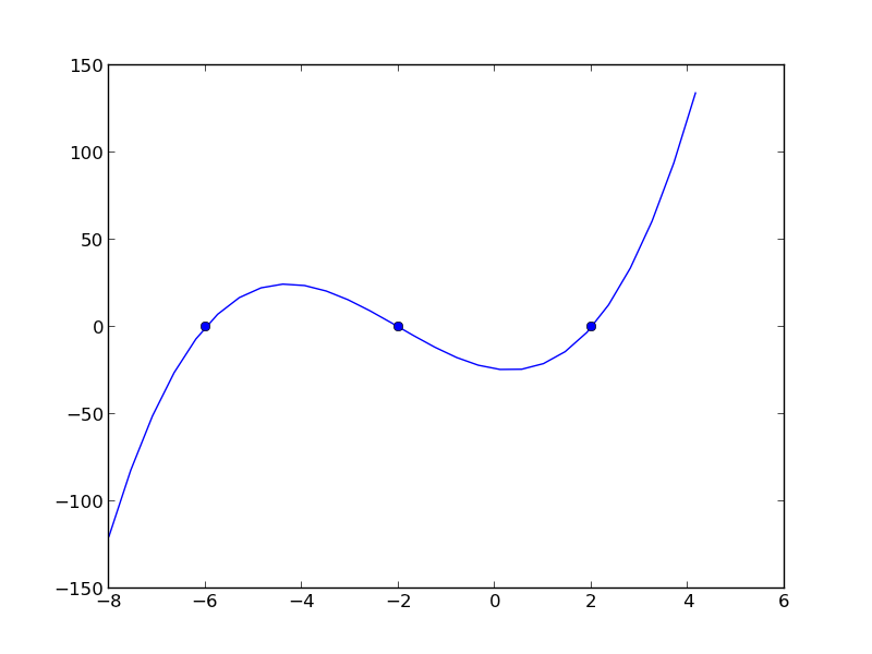
import numpy as np
from scipy.integrate import odeint

def myode(f, x):
    return 3*x**2 + 12*x -4

def event(f, x):
    'an event is when f = 0'
    return f 

# initial conditions
x0 = -8
f0 = -120

# final x-range and step to integrate over.
xf = 4   #final x value
deltax = 0.45 #xstep

# lists to store the results in
X = [x0]
sol = [f0]
e = [event(f0, x0)]
events = []
x2 = x0
# manually integrate at each time step, and check for event sign changes at each step
while x2 <= xf: #stop integrating when we get to xf
    x1 = X[-1]
    x2 = x1 + deltax
    f1 = sol[-1]
    
    f2 = odeint(myode, f1, [x1, x2]) # integrate from x1,f1 to x2,f2
    X += [x2]
    sol += [f2[-1][0]]

    # now evaluate the event at the last position
    e += [event(sol[-1], X[-1])]

    if e[-1] * e[-2] < 0:
        # Event detected where the sign of the event has changed. The
        # event is between xPt = X[-2] and xLt = X[-1]. run a modified bisect
        # function to narrow down to find where event = 0
        xLt = X[-1]
        fLt = sol[-1]
        eLt = e[-1]

        xPt = X[-2]
        fPt = sol[-2]
        ePt = e[-2]

        j = 0
        while j < 100:
            if np.abs(xLt - xPt) < 1e-6:
                # we know the interval to a prescribed precision now.
                # print 'Event found between {0} and {1}'.format(x1t, x2t)
                print 'x = {0}, event = {1}, f = {2}'.format(xLt, eLt, fLt)
                events += [(xLt, fLt)]
                break # and return to integrating

            m = (ePt - eLt)/(xPt - xLt) #slope of line connecting points
                                        #bracketing zero

            #estimated x where the zero is      
            new_x = -ePt / m + xPt

            # now get the new value of the integrated solution at that new x
            f  = odeint(myode, fPt, [xPt, new_x])
            new_f = f[-1][-1]
            new_e = event(new_f, new_x)
                        
            # now check event sign change
            if eLt * new_e > 0:
                xPt = new_x
                fPt = new_f
                ePt = new_e
            else:
                xLt = new_x
                fLt = new_f
                eLt = new_e

            j += 1
        
        
import matplotlib.pyplot as plt
plt.plot(X, sol)

# add event points to the graph
for x,e in events:
    plt.plot(x,e,'bo ')
plt.savefig('images/event-ode-1.png')
x = -6.00000006443, event = -4.63518112781e-15, f = -4.63518112781e-15
x = -1.99999996234, event = -1.40512601554e-15, f = -1.40512601554e-15
x = 1.99999988695, event = -1.11022302463e-15, f = -1.11022302463e-15

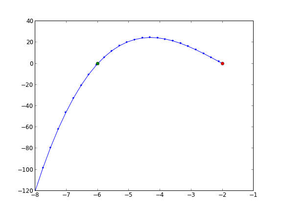
That was a lot of programming to do something like find the roots of the function! Below is an example of using a function coded into pycse to solve the same problem. It is a bit more sophisticated because you can define whether an event is terminal, and the direction of the approach to zero for each event.

from pycse import *
import numpy as np

def myode(f, x):
    return 3*x**2 + 12*x -4

def event1(f, x):
    'an event is when f = 0 and event is decreasing'
    isterminal = True
    direction = -1
    return f, isterminal, direction

def event2(f, x):
    'an event is when f = 0 and increasing'
    isterminal = False
    direction = 1
    return f, isterminal, direction

f0 = -120

xspan = np.linspace(-8, 4)
X, F, TE, YE, IE = odelay(myode, f0, xspan, events=[event1, event2])

import matplotlib.pyplot as plt
plt.plot(X, F, '.-')

# plot the event locations.use a different color for each event
colors = 'rg'

for x,y,i in zip(TE, YE, IE):
    plt.plot([x], [y], 'o', color=colors[i])
    
plt.savefig('images/event-ode-2.png')
plt.show()
print TE, YE, IE
[-6.0000001083101306, -1.9999999635550625] [-3.0871138978483259e-14, -7.7715611723760958e-16] [1, 0]

Copyright (C) 2013 by John Kitchin. See the License for information about copying.

org-mode source

Discuss on Twitter

Integrating the batch reactor mole balance

| categories: ode | tags: reaction engineering

An alternative approach of evaluating an integral is to integrate a differential equation. For the batch reactor, the differential equation that describes conversion as a function of time is:

\(\frac{dX}{dt} = -r_A V/N_{A0}\).

Given a value of initial concentration, or volume and initial number of moles of A, we can integrate this ODE to find the conversion at some later time. We assume that \(X(t=0)=0\). We will integrate the ODE over a time span of 0 to 10,000 seconds.

from scipy.integrate import odeint
import numpy as np
import matplotlib.pyplot as plt

k = 1.0e-3
Ca0 = 1.0  # mol/L

def func(X, t):
    ra = -k * (Ca0 * (1 - X))**2
    return -ra / Ca0

X0 = 0
tspan = np.linspace(0,10000)

sol = odeint(func, X0, tspan)
plt.plot(tspan,sol)
plt.xlabel('Time (sec)')
plt.ylabel('Conversion')
plt.savefig('images/2013-01-06-batch-conversion.png')

You can read off of this figure to find the time required to achieve a particular conversion.

Copyright (C) 2013 by John Kitchin. See the License for information about copying.

org-mode source

Discuss on Twitter

Solving an ode for a specific solution value

| categories: ode | tags:

Matlab post The analytical solution to an ODE is a function, which can be solved to get a particular value, e.g. if the solution to an ODE is y(x) = exp(x), you can solve the solution to find the value of x that makes \(y(x)=2\). In a numerical solution to an ODE we get a vector of independent variable values, and the corresponding function values at those values. To solve for a particular function value we need a different approach. This post will show one way to do that in python.

Given that the concentration of a species A in a constant volume, batch reactor obeys this differential equation \(\frac{dC_A}{dt}=- k C_A^2\) with the initial condition \(C_A(t=0) = 2.3\) mol/L and \(k = 0.23\) L/mol/s, compute the time it takes for \(C_A\) to be reduced to 1 mol/L.

We will get a solution, then create an interpolating function and use fsolve to get the answer.

from scipy.integrate import odeint
from scipy.interpolate import interp1d
from scipy.optimize import fsolve
import numpy as np
import matplotlib.pyplot as plt

k = 0.23
Ca0 = 2.3

def dCadt(Ca, t):
    return -k * Ca**2

tspan = np.linspace(0, 10)

sol = odeint(dCadt, Ca0, tspan)
Ca = sol[:,0]

plt.plot(tspan, Ca)
plt.xlabel('Time (s)')
plt.ylabel('$C_A$ (mol/L)')
plt.savefig('images/ode-specific-1.png')
>>> >>> >>> >>> ... >>> [<matplotlib.lines.Line2D object at 0x1b710d50>]
<matplotlib.text.Text object at 0x1b2f8410>
<matplotlib.text.Text object at 0x1b2fae10>

You can see the solution is near two seconds. Now we create an interpolating function to evaluate the solution. We will plot the interpolating function on a finer grid to make sure it seems reasonable.

ca_func = interp1d(tspan, Ca, 'cubic')

itime = np.linspace(0, 10, 200)

plt.figure()
plt.plot(tspan, Ca, '.')
plt.plot(itime, ca_func(itime), 'b-')

plt.xlabel('Time (s)')
plt.ylabel('$C_A$ (mol/L)')
plt.legend(['solution','interpolated'])
plt.savefig('images/ode-specific-2.png')
plt.show()
>>> >>> >>> <matplotlib.figure.Figure object at 0x1b2dfed0>
[<matplotlib.lines.Line2D object at 0x1c103b90>]
[<matplotlib.lines.Line2D object at 0x1c107050>]
>>> <matplotlib.text.Text object at 0x1c0e65d0>
<matplotlib.text.Text object at 0x1b95bfd0>
<matplotlib.legend.Legend object at 0x1c107550>

that loos pretty reasonable. Now we solve the problem.

tguess = 2.0
tsol, = fsolve(lambda t: 1.0 - ca_func(t), tguess)
print tsol

# you might prefer an explicit function
def func(t):
    return 1.0 - ca_func(t)

tsol2, = fsolve(func, tguess)
print tsol2
>>> 2.4574668235
>>> ... ... >>> 2.4574668235

That is it. Interpolation can provide a simple way to evaluate the numerical solution of an ODE at other values.

For completeness we examine a final way to construct the function. We can actually integrate the ODE in the function to evaluate the solution at the point of interest. If it is not computationally expensive to evaluate the ODE solution this works fine. Note, however, that the ODE will get integrated from 0 to the value t for each iteration of fsolve.

def func(t):
    tspan = [0, t]
    sol = odeint(dCadt, Ca0, tspan)
    return 1.0 - sol[-1]

tsol3, = fsolve(func, tguess)
print tsol3
... ... ... >>> >>> 2.45746688202

Copyright (C) 2013 by John Kitchin. See the License for information about copying.

org-mode source

Discuss on Twitter
« Previous Page