Numerical solution to a simple ode

| categories: ode, interpolation | tags:

Matlab post

Integrate this ordinary differential equation (ode):

$$\frac{dy}{dt} = y(t)$$

over the time span of 0 to 2. The initial condition is y(0) = 1.

to solve this equation, you need to create a function of the form: dydt = f(y, t) and then use one of the odesolvers, e.g. odeint.

import numpy as np
from scipy.integrate import odeint
import matplotlib.pyplot as plt

def fprime(y,t):
    return y

tspan = np.linspace(0, 2)
y0 = 1
ysol = odeint(fprime, y0, tspan)

plt.plot(tspan, ysol, label='numerical solution')
plt.plot(tspan, np.exp(tspan), 'r--', label='analytical solution')
plt.xlabel('time')
plt.ylabel('y(t)')
plt.legend(loc='best')
plt.savefig('images/simple-ode.png')

The numerical and analytical solutions agree.

Now, suppose you want to know at what time is the solution equal to 3? There are several approaches to this, including setting up a solver, or using an event like approach to stop integration at y=3. A simple approach is to use reverse interpolation. We simply reverse the x and y vectors so that y is the independent variable, and we interpolate the corresponding x-value.

import numpy as np
from scipy.integrate import odeint
import matplotlib.pyplot as plt

def fprime(y,t):
    return y

tspan = np.linspace(0, 2)
y0 = 1
ysol = odeint(fprime, y0, tspan)

from scipy.interpolate import interp1d

ip = interp1d(ysol[:,0], tspan) # reverse interpolation
print 'y = 3 at x = {0}'.format(ip(3))
y = 3 at x = 1.09854780564

Copyright (C) 2013 by John Kitchin. See the License for information about copying.

org-mode source

Discuss on Twitter

ODEs with discontinuous forcing functions

| categories: ode | tags:

Matlab post

Adapted from http://archives.math.utk.edu/ICTCM/VOL18/S046/paper.pdf

A mixing tank initially contains 300 g of salt mixed into 1000 L of water. At t=0 min, a solution of 4 g/L salt enters the tank at 6 L/min. At t=10 min, the solution is changed to 2 g/L salt, still entering at 6 L/min. The tank is well stirred, and the tank solution leaves at a rate of 6 L/min. Plot the concentration of salt (g/L) in the tank as a function of time.

A mass balance on the salt in the tank leads to this differential equation: \(\frac{dM_S}{dt} = \nu C_{S,in}(t) - \nu M_S/V\) with the initial condition that \(M_S(t=0)=300\). The wrinkle is that the inlet conditions are not constant.

$$C_{S,in}(t) = \begin{array}{ll} 0 & t \le 0, \\ 4 & 0 < t \le 10, \\ 2 & t > 10. \end{array}$$

import numpy as np
from scipy.integrate import odeint
import matplotlib.pyplot as plt

V = 1000.0 # L
nu = 6.0  # L/min
    
def Cs_in(t):
    'inlet concentration'
    if t < 0:
        Cs = 0.0 # g/L
    elif (t > 0) and (t <= 10):
        Cs = 4.0
    else:
        Cs = 2.0
    return Cs

def mass_balance(Ms, t):
    '$\frac{dM_S}{dt} = \nu C_{S,in}(t) - \nu M_S/V$'
    dMsdt = nu * Cs_in(t) - nu * Ms / V
    return dMsdt

tspan = np.linspace(0.0, 15.0, 50)

M0 = 300.0 # gm salt
Ms = odeint(mass_balance, M0, tspan)

plt.plot(tspan, Ms/V, 'b.-')
plt.xlabel('Time (min)')
plt.ylabel('Salt concentration (g/L)')
plt.savefig('images/ode-discont.png')

You can see the discontinuity in the salt concentration at 10 minutes due to the discontinous change in the entering salt concentration.

Copyright (C) 2013 by John Kitchin. See the License for information about copying.

org-mode source

Discuss on Twitter

Phase portraits of a system of ODEs

| categories: ode, math | tags:

Matlab post An undamped pendulum with no driving force is described by

$$ y'' + sin(y) = 0$$

We reduce this to standard matlab form of a system of first order ODEs by letting \(y_1 = y\) and \(y_2=y_1'\). This leads to:

\(y_1' = y_2\)

\(y_2' = -sin(y_1)\)

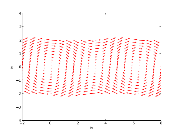
The phase portrait is a plot of a vector field which qualitatively shows how the solutions to these equations will go from a given starting point. here is our definition of the differential equations:

To generate the phase portrait, we need to compute the derivatives \(y_1'\) and \(y_2'\) at \(t=0\) on a grid over the range of values for \(y_1\) and \(y_2\) we are interested in. We will plot the derivatives as a vector at each (y1, y2) which will show us the initial direction from each point. We will examine the solutions over the range -2 < y1 < 8, and -2 < y2 < 2 for y2, and create a grid of 20 x 20 points.

import numpy as np
import matplotlib.pyplot as plt

def f(Y, t):
    y1, y2 = Y
    return [y2, -np.sin(y1)]

y1 = np.linspace(-2.0, 8.0, 20)
y2 = np.linspace(-2.0, 2.0, 20)

Y1, Y2 = np.meshgrid(y1, y2)

t = 0

u, v = np.zeros(Y1.shape), np.zeros(Y2.shape)

NI, NJ = Y1.shape

for i in range(NI):
    for j in range(NJ):
        x = Y1[i, j]
        y = Y2[i, j]
        yprime = f([x, y], t)
        u[i,j] = yprime[0]
        v[i,j] = yprime[1]
     

Q = plt.quiver(Y1, Y2, u, v, color='r')

plt.xlabel('$y_1$')
plt.ylabel('$y_2$')
plt.xlim([-2, 8])
plt.ylim([-4, 4])
plt.savefig('images/phase-portrait.png')
>>> ... >>> >>> >>> >>> >>> >>> ... ... ... >>> >>> <matplotlib.text.Text object at 0xbcfd290>
<matplotlib.text.Text object at 0xbd14750>
(-2, 8)
(-4, 4)

Let us plot a few solutions on the vector field. We will consider the solutions where y1(0)=0, and values of y2(0) = [0 0.5 1 1.5 2 2.5], in otherwords we start the pendulum at an angle of zero, with some angular velocity.

from scipy.integrate import odeint

for y20 in [0, 0.5, 1, 1.5, 2, 2.5]:
    tspan = np.linspace(0, 50, 200)
    y0 = [0.0, y20]
    ys = odeint(f, y0, tspan)
    plt.plot(ys[:,0], ys[:,1], 'b-') # path
    plt.plot([ys[0,0]], [ys[0,1]], 'o') # start
    plt.plot([ys[-1,0]], [ys[-1,1]], 's') # end
    

plt.xlim([-2, 8])
plt.savefig('images/phase-portrait-2.png')
plt.show()
>>> ... ... ... [<matplotlib.lines.Line2D object at 0xbc0dbd0>]
[<matplotlib.lines.Line2D object at 0xc135050>]
[<matplotlib.lines.Line2D object at 0xbd1a450>]
[<matplotlib.lines.Line2D object at 0xbd1a1d0>]
[<matplotlib.lines.Line2D object at 0xb88aa10>]
[<matplotlib.lines.Line2D object at 0xb88a5d0>]
[<matplotlib.lines.Line2D object at 0xc14e410>]
[<matplotlib.lines.Line2D object at 0xc14ed90>]
[<matplotlib.lines.Line2D object at 0xc2c5290>]
[<matplotlib.lines.Line2D object at 0xbea4bd0>]
[<matplotlib.lines.Line2D object at 0xbea4d50>]
[<matplotlib.lines.Line2D object at 0xbc401d0>]
[<matplotlib.lines.Line2D object at 0xc2d1190>]
[<matplotlib.lines.Line2D object at 0xc2f3e90>]
[<matplotlib.lines.Line2D object at 0xc2f3bd0>]
[<matplotlib.lines.Line2D object at 0xc2e4790>]
[<matplotlib.lines.Line2D object at 0xc2e0a90>]
[<matplotlib.lines.Line2D object at 0xc2c7390>]
(-2, 8)

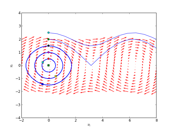
What do these figures mean? For starting points near the origin, and small velocities, the pendulum goes into a stable limit cycle. For others, the trajectory appears to fly off into y1 space. Recall that y1 is an angle that has values from \(-\pi\) to \(\pi\). The y1 data in this case is not wrapped around to be in this range.

Copyright (C) 2013 by John Kitchin. See the License for information about copying.

org-mode source

Discuss on Twitter

Plug flow reactor with a pressure drop

| categories: ode | tags: fluids, reaction engineering

If there is a pressure drop in a plug flow reactor, 1 there are two equations needed to determine the exit conversion: one for the conversion, and one from the pressure drop.

\begin{eqnarray} \frac{dX}{dW} &=& \frac{k'}{F_A0} \left ( \frac{1-X}{1 + \epsilon X} \right) y\\ \frac{dX}{dy} &=& -\frac{\alpha (1 + \epsilon X)}{2y} \end{eqnarray}

Here is how to integrate these equations numerically in python.

import numpy as np
from scipy.integrate import odeint
import matplotlib.pyplot as plt

kprime = 0.0266
Fa0 = 1.08
alpha = 0.0166
epsilon = -0.15

def dFdW(F, W):
    'set of ODEs to integrate'
    X = F[0]
    y = F[1]
    dXdW = kprime / Fa0 * (1-X) / (1 + epsilon*X) * y
    dydW = -alpha * (1 + epsilon * X) / (2 * y)
    return [dXdW, dydW]

Wspan = np.linspace(0,60)
X0 = 0.0
y0 = 1.0
F0 = [X0, y0]
sol = odeint(dFdW, F0, Wspan)

# now plot the results
plt.plot(Wspan, sol[:,0], label='Conversion')
plt.plot(Wspan, sol[:,1], 'g--', label='y=$P/P_0$')
plt.legend(loc='best')
plt.xlabel('Catalyst weight (lb_m)')
plt.savefig('images/2013-01-08-pdrop.png')

Here is the resulting figure.

Copyright (C) 2013 by John Kitchin. See the License for information about copying.

org-mode source

Discuss on Twitter

Integrating the batch reactor mole balance

| categories: ode | tags: reaction engineering

An alternative approach of evaluating an integral is to integrate a differential equation. For the batch reactor, the differential equation that describes conversion as a function of time is:

\(\frac{dX}{dt} = -r_A V/N_{A0}\).

Given a value of initial concentration, or volume and initial number of moles of A, we can integrate this ODE to find the conversion at some later time. We assume that \(X(t=0)=0\). We will integrate the ODE over a time span of 0 to 10,000 seconds.

from scipy.integrate import odeint
import numpy as np
import matplotlib.pyplot as plt

k = 1.0e-3
Ca0 = 1.0  # mol/L

def func(X, t):
    ra = -k * (Ca0 * (1 - X))**2
    return -ra / Ca0

X0 = 0
tspan = np.linspace(0,10000)

sol = odeint(func, X0, tspan)
plt.plot(tspan,sol)
plt.xlabel('Time (sec)')
plt.ylabel('Conversion')
plt.savefig('images/2013-01-06-batch-conversion.png')

You can read off of this figure to find the time required to achieve a particular conversion.

Copyright (C) 2013 by John Kitchin. See the License for information about copying.

org-mode source

Discuss on Twitter
« Previous Page -- Next Page »