Gibbs energy minimization and the NIST webbook

| categories: optimization | tags: thermodynamics

Matlab post In Post 1536 we used the NIST webbook to compute a temperature dependent Gibbs energy of reaction, and then used a reaction extent variable to compute the equilibrium concentrations of each species for the water gas shift reaction.

Today, we look at the direct minimization of the Gibbs free energy of the species, with no assumptions about stoichiometry of reactions. We only apply the constraint of conservation of atoms. We use the NIST Webbook to provide the data for the Gibbs energy of each species.

As a reminder we consider equilibrium between the species \(CO\), \(H_2O\), \(CO_2\) and \(H_2\), at 1000K, and 10 atm total pressure with an initial equimolar molar flow rate of \(CO\) and \(H_2O\).

import numpy as np

T = 1000  # K
R = 8.314e-3 # kJ/mol/K

P = 10.0 # atm, this is the total pressure in the reactor
Po = 1.0 # atm, this is the standard state pressure

We are going to store all the data and calculations in vectors, so we need to assign each position in the vector to a species. Here are the definitions we use in this work.

1  CO
2  H2O
3  CO2
4  H2
species = ['CO', 'H2O', 'CO2', 'H2']

# Heats of formation at 298.15 K

Hf298 = [
    -110.53,  # CO
    -241.826, # H2O
    -393.51,  # CO2
       0.0]   # H2

# Shomate parameters for each species
#           A          B           C          D          E            F          G       H
WB = [[25.56759,  6.096130,     4.054656,  -2.671301,  0.131021, -118.0089, 227.3665,   -110.5271],  # CO
      [30.09200,  6.832514,     6.793435,  -2.534480,  0.082139, -250.8810, 223.3967,   -241.8264],  # H2O
      [24.99735,  55.18696,   -33.69137,    7.948387, -0.136638, -403.6075, 228.2431,   -393.5224],  # CO2
      [33.066178, -11.363417,  11.432816,  -2.772874, -0.158558, -9.980797, 172.707974,    0.0]]     # H2

WB = np.array(WB)

# Shomate equations
t = T/1000
T_H = np.array([t,  t**2 / 2.0, t**3 / 3.0, t**4 / 4.0, -1.0 / t, 1.0, 0.0, -1.0])
T_S = np.array([np.log(t), t,  t**2 / 2.0,  t**3 / 3.0, -1.0 / (2.0 * t**2), 0.0, 1.0, 0.0])

H = np.dot(WB, T_H)        # (H - H_298.15) kJ/mol
S = np.dot(WB, T_S/1000.0) # absolute entropy kJ/mol/K

Gjo = Hf298 + H - T*S      # Gibbs energy of each component at 1000 K

Now, construct the Gibbs free energy function, accounting for the change in activity due to concentration changes (ideal mixing).

def func(nj):
    nj = np.array(nj)
    Enj = np.sum(nj);
    Gj =  Gjo / (R * T) + np.log(nj / Enj * P / Po)
    return np.dot(nj, Gj)

We impose the constraint that all atoms are conserved from the initial conditions to the equilibrium distribution of species. These constraints are in the form of \(A_{eq} n = b_{eq}\), where \(n\) is the vector of mole numbers for each species.

Aeq = np.array([[ 1,    0,    1,    0],  # C balance
                [ 1,    1,    2,    0],  # O balance
                [ 0,    2,    0,    2]]) # H balance

# equimolar feed of 1 mol H2O and 1 mol CO
beq = np.array([1,  # mol C fed
                2,  # mol O fed
                2]) # mol H fed

def ec1(nj):
    'conservation of atoms constraint'
    return np.dot(Aeq, nj) - beq

Now we are ready to solve the problem.

from scipy.optimize import fmin_slsqp

n0 = [0.5, 0.5, 0.5, 0.5]  # initial guesses
N = fmin_slsqp(func, n0, f_eqcons=ec1)
print N
>>> >>> Optimization terminated successfully.    (Exit mode 0)
            Current function value: -91.204832308
            Iterations: 2
            Function evaluations: 13
            Gradient evaluations: 2
[ 0.45502309  0.45502309  0.54497691  0.54497691]

1 Compute mole fractions and partial pressures

The pressures here are in good agreement with the pressures found by other methods. The minor disagreement (in the third or fourth decimal place) is likely due to convergence tolerances in the different algorithms used.

yj = N / np.sum(N)
Pj = yj * P

for s, y, p in zip(species, yj, Pj):
    print '{0:10s}: {1:1.2f} {2:1.2f}'.format(s, y, p)
>>> >>> ... ... CO        : 0.23 2.28
H2O       : 0.23 2.28
CO2       : 0.27 2.72
H2        : 0.27 2.72

2 Computing equilibrium constants

We can compute the equilibrium constant for the reaction \(CO + H_2O \rightleftharpoons CO_2 + H_2\). Compared to the value of K = 1.44 we found at the end of Post 1536 , the agreement is excellent. Note, that to define an equilibrium constant it is necessary to specify a reaction, even though it is not necessary to even consider a reaction to obtain the equilibrium distribution of species!

nuj = np.array([-1, -1, 1, 1])  # stoichiometric coefficients of the reaction
K = np.prod(yj**nuj)
print K
>>> 1.43446295961

Copyright (C) 2013 by John Kitchin. See the License for information about copying.
org-mode source

Discuss on Twitter

Finding equilibrium composition by direct minimization of Gibbs free energy on mole numbers

| categories: optimization | tags: thermodynamics

Matlab post Adapted from problem 4.5 in Cutlip and Shacham Ethane and steam are fed to a steam cracker at a total pressure of 1 atm and at 1000K at a ratio of 4 mol H2O to 1 mol ethane. Estimate the equilibrium distribution of products (CH4, C2H4, C2H2, CO2, CO, O2, H2, H2O, and C2H6).

Solution method: We will construct a Gibbs energy function for the mixture, and obtain the equilibrium composition by minimization of the function subject to elemental mass balance constraints.

import numpy as np

R = 0.00198588 # kcal/mol/K
T = 1000 # K

species = ['CH4', 'C2H4', 'C2H2', 'CO2', 'CO', 'O2', 'H2', 'H2O', 'C2H6']

# $G_^\circ for each species. These are the heats of formation for each
# species.
Gjo = np.array([4.61, 28.249, 40.604, -94.61, -47.942, 0, 0, -46.03, 26.13]) # kcal/mol

1 The Gibbs energy of a mixture

We start with \(G=\sum\limits_j n_j \mu_j\). Recalling that we define \(\mu_j = G_j^\circ + RT \ln a_j\), and in the ideal gas limit, \(a_j = y_j P/P^\circ\), and that \(y_j = \frac{n_j}{\sum n_j}\). Since in this problem, P = 1 atm, this leads to the function \(\frac{G}{RT} = \sum\limits_{j=1}^n n_j\left(\frac{G_j^\circ}{RT} + \ln \frac{n_j}{\sum n_j}\right)\).

import numpy as np

def func(nj):
    nj = np.array(nj)
    Enj = np.sum(nj);
    G = np.sum(nj * (Gjo / R / T + np.log(nj / Enj)))
    return G

2 Linear equality constraints for atomic mass conservation

The total number of each type of atom must be the same as what entered the reactor. These form equality constraints on the equilibrium composition. We express these constraints as: \(A_{eq} n = b\) where \(n\) is a vector of the moles of each species present in the mixture. CH4 C2H4 C2H2 CO2 CO O2 H2 H2O C2H6

Aeq = np.array([[0,   0,    0,   2,   1,  2,  0,  1,   0],      # oxygen balance
                [4,   4,    2,   0,   0,  0,  2,  2,   6],      # hydrogen balance
                [1,   2,    2,   1,   1,  0,  0,  0,   2]])     # carbon balance

# the incoming feed was 4 mol H2O and 1 mol ethane
beq = np.array([4,  # moles of oxygen atoms coming in
                14, # moles of hydrogen atoms coming in
                2]) # moles of carbon atoms coming in

def ec1(n):
    'equality constraint'
    return np.dot(Aeq, n) - beq

def ic1(n):
    '''inequality constraint
       all n>=0
    '''   
    return n

Now we solve the problem.

# initial guess suggested in the example
n0 = [1e-3, 1e-3, 1e-3, 0.993, 1.0, 1e-4, 5.992, 1.0, 1e-3] 

n0 = [0.066, 8.7e-08, 2.1e-14, 0.545, 1.39, 5.7e-14, 5.346, 1.521, 1.58e-7]

from scipy.optimize import fmin_slsqp

X = fmin_slsqp(func, n0, f_eqcons=ec1,f_ieqcons=ic1, iter=300, acc=1e-12)

for s,x in zip(species, X):
    print '{0:10s} {1:1.4g}'.format(s, x)

# check that constraints were met
print np.dot(Aeq, X) - beq
print np.all( np.abs( np.dot(Aeq, X) - beq) < 1e-12)
>>> >>> >>> >>> >>> >>> Optimization terminated successfully.    (Exit mode 0)
            Current function value: -104.403951524
            Iterations: 16
            Function evaluations: 193
            Gradient evaluations: 15
>>> ... ... CH4        0.06644
C2H4       9.48e-08
C2H2       1.487e-13
CO2        0.545
CO         1.389
O2         3.096e-13
H2         5.346
H2O        1.521
C2H6       1.581e-07
... [  0.00000000e+00   0.00000000e+00   4.44089210e-16]
True

I found it necessary to tighten the accuracy parameter to get pretty good matches to the solutions found in Matlab. It was also necessary to increase the number of iterations. Even still, not all of the numbers match well, especially the very small numbers. You can, however, see that the constraints were satisfied pretty well.

Interestingly there is a distribution of products! That is interesting because only steam and ethane enter the reactor, but a small fraction of methane is formed! The main product is hydrogen. The stoichiometry of steam reforming is ideally \(C_2H_6 + 4H_2O \rightarrow 2CO_2 + 7 H2\). Even though nearly all the ethane is consumed, we do not get the full yield of hydrogen. It appears that another equilibrium, one between CO, CO2, H2O and H2, may be limiting that, since the rest of the hydrogen is largely in the water. It is also of great importance that we have not said anything about reactions, i.e. how these products were formed.

The water gas shift reaction is: \(CO + H_2O \rightleftharpoons CO_2 + H_2\). We can compute the Gibbs free energy of the reaction from the heats of formation of each species. Assuming these are the formation energies at 1000K, this is the reaction free energy at 1000K.

G_wgs = Gjo[3] + Gjo[6] - Gjo[4] - Gjo[7]
print G_wgs

K = np.exp(-G_wgs / (R*T))
print K
-0.638
>>> >>> 1.37887528109

3 Equilibrium constant based on mole numbers

One normally uses activities to define the equilibrium constant. Since there are the same number of moles on each side of the reaction all factors that convert mole numbers to activity, concentration or pressure cancel, so we simply consider the ratio of mole numbers here.

print (X[3] * X[6]) / (X[4] * X[7])
1.37887525547

This is very close to the equilibrium constant computed above.

Clearly, there is an equilibrium between these species that prevents the complete reaction of steam reforming.

4 Summary

This is an appealing way to minimize the Gibbs energy of a mixture. No assumptions about reactions are necessary, and the constraints are easy to identify. The Gibbs energy function is especially easy to code.

Copyright (C) 2014 by John Kitchin. See the License for information about copying.
org-mode source

Org-mode version = 8.2.7c

Discuss on Twitter

Meet the steam tables

| categories: uncategorized | tags: steam, thermodynamics

Matlab post

We will use the iapws module. Install it like this:

pip install iapws

Problem statement: A Rankine cycle operates using steam with the condenser at 100 degC, a pressure of 3.0 MPa and temperature of 600 degC in the boiler. Assuming the compressor and turbine operate reversibly, estimate the efficiency of the cycle.

Starting point in the Rankine cycle in condenser.

we have saturated liquid here, and we get the thermodynamic properties for the given temperature. In this python module, these properties are all in attributes of an IAPWS object created at a set of conditions.

1 Starting point in the Rankine cycle in condenser.

We have saturated liquid here, and we get the thermodynamic properties for the given temperature.

from iapws import IAPWS97

T1 = 100 + 273.15 #in K

sat_liquid1  = IAPWS97(T=T1, x=0) # x is the steam quality. 0 = liquid

P1 = sat_liquid1.P
s1 = sat_liquid1.s
h1 = sat_liquid1.h
v1 = sat_liquid1.v

2 Isentropic compression of liquid to point 2

The final pressure is given, and we need to compute the new temperatures, and enthalpy.

P2 = 3.0 # MPa
s2 = s1 # this is what isentropic means

sat_liquid2 = IAPWS97(P=P2, s=s1)
T2, = sat_liquid2.T
h2 = sat_liquid2.h

# work done to compress liquid. This is an approximation, since the
# volume does change a little with pressure, but the overall work here
# is pretty small so we neglect the volume change.
WdotP = v1*(P2 - P1);
print
print('The compressor work is: {0:1.4f} kJ/kg'.format(WdotP))
>>> >>> >>> >>> >>> >>> ... ... ... >>>
The compressor work is: 0.0030 kJ/kg

The compression work is almost negligible. This number is 1000 times smaller than we computed with Xsteam. I wonder what the units of v1 actually are.

3 Isobaric heating to T3 in boiler where we make steam

T3 = 600 + 273.15 # K
P3 = P2 # definition of isobaric
steam = IAPWS97(P=P3, T=T3)

h3 = steam.h
s3 = steam.s

Qb, = h3 - h2 # heat required to make the steam

print
print 'The boiler heat duty is: {0:1.2f} kJ/kg'.format(Qb)
>>> >>> >>> >>> >>> >>> >>> >>>
The boiler heat duty is: 3260.69 kJ/kg

4 Isentropic expansion through turbine to point 4

steam =  IAPWS97(P=P1, s=s3)
T4, = steam.T
h4 = steam.h
s4 = s3 # isentropic
Qc, = h4 - h1 # work required to cool from T4 to T1
print 
print 'The condenser heat duty is {0:1.2f} kJ/kg'.format(Qc)
>>> >>> >>> >>>
The condenser heat duty is 2317.00 kJ/kg

5 To get from point 4 to point 1

WdotTurbine, = h4 - h3 # work extracted from the expansion
print('The turbine work is: {0:1.2f} kJ/kg'.format(WdotTurbine))
The turbine work is: -946.71 kJ/kg

6 Efficiency

This is a ratio of the work put in to make the steam, and the net work obtained from the turbine. The answer here agrees with the efficiency calculated in Sandler on page 135.

eta = -(WdotTurbine - WdotP) / Qb
print('The overall efficiency is {0:1.2%}.'.format(eta))
The overall efficiency is 29.03%.

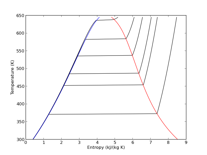
7 Entropy-temperature chart

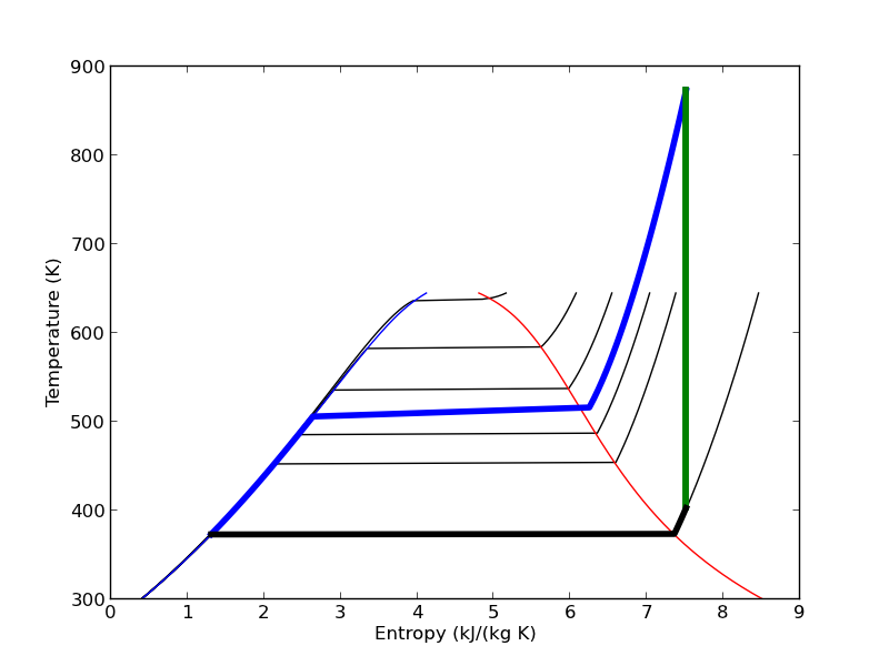
The IAPWS module makes it pretty easy to generate figures of the steam tables. Here we generate an entropy-Temperature graph. We do this to illustrate the path of the Rankine cycle. We need to compute the values of steam entropy for a range of pressures and temperatures.

import numpy as np
import matplotlib.pyplot as plt

plt.figure()
plt.clf()
T = np.linspace(300, 372+273, 200) # range of temperatures
for P in [0.1, 1, 2, 5, 10, 20]: #MPa
    steam = [IAPWS97(T=t, P=P) for t in T]
    S = [s.s for s in steam]
    plt.plot(S, T, 'k-')

# saturated vapor and liquid entropy lines
svap = [s.s for s in [IAPWS97(T=t, x=1) for t in T]]
sliq = [s.s for s in [IAPWS97(T=t, x=0) for t in T]]

plt.plot(svap, T, 'r-')
plt.plot(sliq, T, 'b-')

plt.xlabel('Entropy (kJ/(kg K)')
plt.ylabel('Temperature (K)')
plt.savefig('images/iawps-steam.png')
>>> >>> <matplotlib.figure.Figure object at 0x000000000638BC18>
>>> >>> ... ... ... ... [<matplotlib.lines.Line2D object at 0x0000000007F9C208>]
[<matplotlib.lines.Line2D object at 0x0000000007F9C400>]
[<matplotlib.lines.Line2D object at 0x0000000007F9C8D0>]
[<matplotlib.lines.Line2D object at 0x0000000007F9CD30>]
[<matplotlib.lines.Line2D object at 0x0000000007F9E1D0>]
[<matplotlib.lines.Line2D object at 0x0000000007F9E630>]
... >>> >>> >>> [<matplotlib.lines.Line2D object at 0x0000000001FDCEB8>]
[<matplotlib.lines.Line2D object at 0x0000000007F9EA90>]
>>> <matplotlib.text.Text object at 0x0000000007F7BE48>
<matplotlib.text.Text object at 0x0000000007F855F8>

We can plot our Rankine cycle path like this. We compute the entropies along the non-isentropic paths.

T23 = np.linspace(T2, T3)
S23 = [s.s for s in [IAPWS97(P=P2, T=t) for t in T23]]

T41 = np.linspace(T4, T1 - 0.01) # subtract a tiny bit to make sure we get a liquid
S41 = [s.s for s in [IAPWS97(P=P1, T=t) for t in T41]]

And then we plot the paths.

plt.plot([s1, s2], [T1, T2], 'r-', lw=4) # Path 1 to 2
plt.plot(S23, T23, 'b-', lw=4) # path from 2 to 3 is isobaric
plt.plot([s3, s4], [T3, T4], 'g-', lw=4) # path from 3 to 4 is isentropic
plt.plot(S41, T41, 'k-', lw=4) # and from 4 to 1 is isobaric
plt.savefig('images/iawps-steam-2.png')
plt.savefig('images/iawps-steam-2.svg')
[<matplotlib.lines.Line2D object at 0x0000000008350908>]
[<matplotlib.lines.Line2D object at 0x00000000083358D0>]
[<matplotlib.lines.Line2D object at 0x000000000835BEB8>]
[<matplotlib.lines.Line2D object at 0x0000000008357160>]

8 Summary

This was an interesting exercise. On one hand, the tedium of interpolating the steam tables is gone. On the other hand, you still have to know exactly what to ask for to get an answer that is correct. The iapws interface is a little clunky, and takes some getting used to. It does not seem as robust as the Xsteam module I used in Matlab.

Copyright (C) 2013 by John Kitchin. See the License for information about copying.
org-mode source

Discuss on Twitter

Reading parameter database text files in python

| categories: io | tags: thermodynamics

Matlab post

The datafile at http://terpconnect.umd.edu/~nsw/ench250/antoine.dat (dead link) contains data that can be used to estimate the vapor pressure of about 700 pure compounds using the Antoine equation

The data file has the following contents:

Antoine Coefficients
  log(P) = A-B/(T+C) where P is in mmHg and T is in Celsius
Source of data: Yaws and Yang (Yaws, C.  L.  and Yang, H.  C.,
"To estimate vapor pressure easily. antoine coefficients relate vapor pressure to temperature for almost 700 major organic compounds", Hydrocarbon Processing, 68(10), p65-68, 1989.

ID  formula  compound name                  A       B       C     Tmin Tmax ??    ?
-----------------------------------------------------------------------------------
  1 CCL4     carbon-tetrachloride        6.89410 1219.580 227.170  -20  101 Y2    0
  2 CCL3F    trichlorofluoromethane      6.88430 1043.010 236.860  -33   27 Y2    0
  3 CCL2F2   dichlorodifluoromethane     6.68619  782.072 235.377 -119  -30 Y6    0

To use this data, you find the line that has the compound you want, and read off the data. You could do that manually for each component you want but that is tedious, and error prone. Today we will see how to retrieve the file, then read the data into python to create a database we can use to store and retrieve the data.

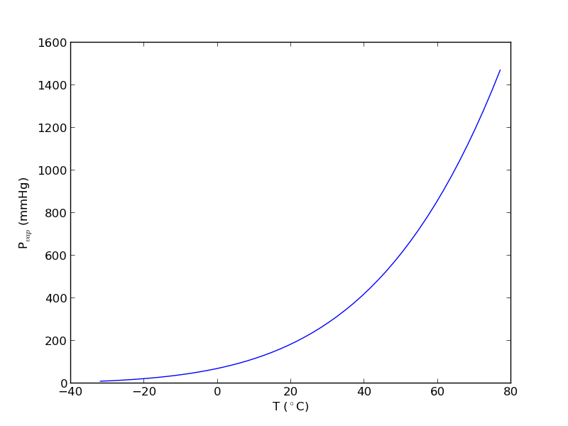
We will use the data to find the temperature at which the vapor pressure of acetone is 400 mmHg.

We use numpy.loadtxt to read the file, and tell the function the format of each column. This creates a special kind of record array which we can access data by field name.

import numpy as np
import matplotlib.pyplot as plt

data = np.loadtxt('data/antoine_data.dat',
                  dtype=[('id', np.int),
                         ('formula', 'S8'),
                         ('name', 'S28'),
                         ('A', np.float),
                         ('B', np.float),
                         ('C', np.float),
                         ('Tmin', np.float),
                         ('Tmax', np.float),
                         ('??', 'S4'),
                         ('?', 'S4')],
                  skiprows=7)

names = data['name']

acetone, = data[names == 'acetone']

# for readability we unpack the array into variables
id, formula, name, A, B, C, Tmin, Tmax, u1, u2 = acetone

T = np.linspace(Tmin, Tmax)
P = 10**(A - B / ( T + C))
plt.plot(T, P)
plt.xlabel('T ($^\circ$C)')
plt.ylabel('P$_{vap}$ (mmHg)')

# Find T at which Pvap = 400 mmHg
# from our graph we might guess T ~ 40 ^{\circ}C

def objective(T):
    return 400 - 10**(A - B / (T + C))

from scipy.optimize import fsolve
Tsol, = fsolve(objective, 40)
print Tsol
print 'The vapor pressure is 400 mmHg at T = {0:1.1f} degC'.format(Tsol)

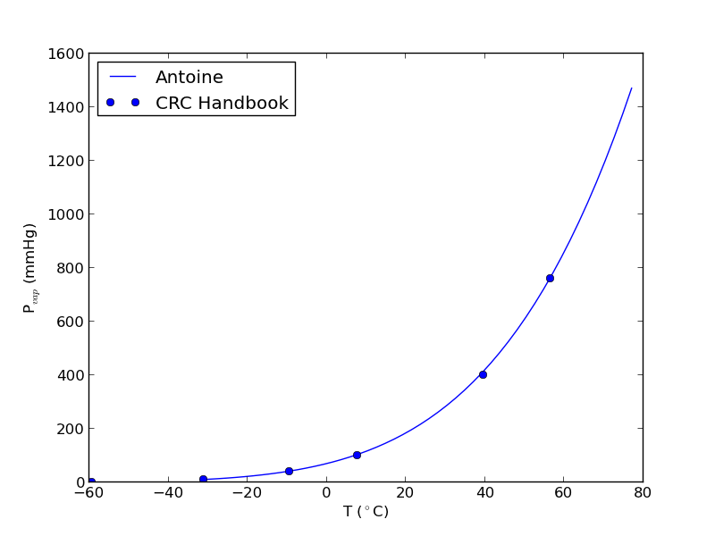
#Plot CRC data http://en.wikipedia.org/wiki/Acetone_%28data_page%29#Vapor_pressure_of_liquid
# We only include the data for the range where the Antoine fit is valid.

Tcrc  = [-59.4,         -31.1,  -9.4,   7.7,    39.5,   56.5]
Pcrc = [        1,      10,     40,     100,    400,    760]

plt.plot(Tcrc, Pcrc, 'bo')
plt.legend(['Antoine','CRC Handbook'], loc='best')
plt.savefig('images/antoine-2.png')
38.6138198197
The vapor pressure is 400 mmHg at T = 38.6 degC

This result is close to the value reported here (39.5 degC), from the CRC Handbook. The difference is probably that the value reported in the CRC is an actual experimental number.

Copyright (C) 2013 by John Kitchin. See the License for information about copying.
org-mode source

Discuss on Twitter

Calculating a bubble point pressure of a mixture

| categories: nonlinear algebra | tags: thermodynamics

Matlab post

Adapted from http://terpconnect.umd.edu/~nsw/ench250/bubpnt.htm (dead link)

We previously learned to read a datafile containing lots of Antoine coefficients into a database, and use the coefficients to estimate vapor pressure of a single compound. Here we use those coefficents to compute a bubble point pressure of a mixture.

The bubble point is the temperature at which the sum of the component vapor pressures is equal to the the total pressure. This is where a bubble of vapor will first start forming, and the mixture starts to boil.

Consider an equimolar mixture of benzene, toluene, chloroform, acetone and methanol. Compute the bubble point at 760 mmHg, and the gas phase composition. The gas phase composition is given by: \(y_i = x_i*P_i/P_T\).

import numpy as np
from scipy.optimize import fsolve

# load our thermodynamic data
data = np.loadtxt('data/antoine_data.dat',
                  dtype=[('id', np.int),
                         ('formula', 'S8'),
                         ('name', 'S28'),
                         ('A', np.float),
                         ('B', np.float),
                         ('C', np.float),
                         ('Tmin', np.float),
                         ('Tmax', np.float),
                         ('??', 'S4'),
                         ('?', 'S4')],
                  skiprows=7)

compounds = ['benzene', 'toluene', 'chloroform', 'acetone', 'methanol']

# extract the data we want
A = np.array([data[data['name'] == x]['A'][0] for x in compounds])
B = np.array([data[data['name'] == x]['B'][0] for x in compounds])
C = np.array([data[data['name'] == x]['C'][0] for x in compounds])
Tmin = np.array([data[data['name'] == x]['Tmin'][0] for x in compounds])
Tmax = np.array([data[data['name'] == x]['Tmax'][0] for x in compounds])


# we have an equimolar mixture
x = np.array([0.2, 0.2, 0.2, 0.2, 0.2])

# Given a T, we can compute the pressure of each species like this:

T = 67 # degC
P = 10**(A - B / (T + C))
print P
print np.dot(x, P)  # total mole-fraction weighted pressure

Tguess = 67
Ptotal = 760

def func(T):
    P = 10**(A - B / (T + C))
    return Ptotal - np.dot(x, P)
    
Tbubble, = fsolve(func, Tguess)

print 'The bubble point is {0:1.2f} degC'.format(Tbubble)

# double check answer is in a valid T range
if np.any(Tbubble < Tmin) or np.any(Tbubble > Tmax):
    print 'T_bubble is out of range!'

# print gas phase composition
y = x * 10**(A - B / (Tbubble + C))/Ptotal

for cmpd, yi in zip(compounds, y):
    print 'y_{0:<10s} = {1:1.3f}'.format(cmpd, yi)
[  498.4320267    182.16010994   898.31061294  1081.48181768   837.88860027]
699.654633507
The bubble point is 69.46 degC
y_benzene    = 0.142
y_toluene    = 0.053
y_chloroform = 0.255
y_acetone    = 0.308
y_methanol   = 0.242

Copyright (C) 2013 by John Kitchin. See the License for information about copying.

org-mode source

Discuss on Twitter
Next Page ยป