Uncertainty in implicit functions

| categories: statistics | tags:

Suppose we have an equation \(y = e^{a y}\) that we want to solve, where \(a\) is a constant with some uncertainty. What is the uncertainty in the solution \(y\)?

Finding a solution is not difficult. The uncertainty in the solution, however, is not easy, since we do not have an explicit function to propagate errors through. Let us examine the solution first.

import numpy as np
from scipy.optimize import fsolve

a = 0.20

def f(y):
    return y - np.exp(a * y)

sol, = fsolve(f, 1)
print sol
1.2958555091

A way to estimate the uncertainty is by Monte Carlo simulation. We solve the equation many times, using values sampled from the uncertainty distribution. Here we assume that the \(a\) parameter is normally distributed with an average of 0.2 and a std deviation of 0.02. We solve the equation 10000 times for different values of \(a\) sampled according to the normal distribution. That gives us a distribution of solutions that we can do statistical analysis of to get the average and std deviation.

import numpy as np
from scipy.optimize import fsolve
N = 10000

A = np.random.normal(0.2, 0.02, size=N)

sol = np.zeros(A.shape)

for i, a in enumerate(A):
    s, = fsolve(lambda y:y - np.exp(a * y), 1)
    sol[i] = s

ybar = np.mean(sol)
s_y = np.std(sol)

print ybar, s_y, s_y / ybar

import matplotlib.pyplot as plt
count, bins, ignored = plt.hist(sol)
plt.savefig('images/implicit-uncertainty.png')
1.29887470397 0.0465110111613 0.0358086973433

We get approximately the same answer, and you can see here the distribution of solution values is not quite normal. We compute the standard deviation anyway, and find the standard deviation is about 3.6%. It would be nice to have some analytical method to estimate this uncertainty. So far I have not figured that out.

This method could have relevance in estimating the uncertainty in the friction factor for turbulent flow (\(Re > 2100\)). In that case we have the implicit equation \(\frac{1}{\sqrt{f_F}}=4.0 \log(Re \sqrt{f_F})-0.4\). Uncertainties in the Re number would lead to uncertainties in the friction factor. Whether those uncertainties are larger than the uncertainties from the original correlation would require some investigation.

Copyright (C) 2013 by John Kitchin. See the License for information about copying.

org-mode source
Discuss on Twitter

Interacting with Excel in python

| categories: programming | tags:

Matlab post

There will be times it is convenient to either read data from Excel, or write data to Excel. This is possible in python (http://www.python-excel.org/). You may also look at (https://bitbucket.org/ericgazoni/openpyxl/wiki/Home).

import xlrd

wb = xlrd.open_workbook('data/example.xlsx')
sh1 = wb.sheet_by_name(u'Sheet1')

print sh1.col_values(0)  # column 0
print sh1.col_values(1)  # column 1

sh2 = wb.sheet_by_name(u'Sheet2')

x = sh2.col_values(0)  # column 0
y = sh2.col_values(1)  # column 1

import matplotlib.pyplot as plt
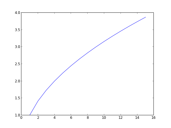
plt.plot(x, y)
plt.savefig('images/excel-1.png')
[u'value', u'function']
[2.0, 3.0]

1 Writing Excel workbooks

Writing data to Excel sheets is pretty easy. Note, however, that this overwrites the worksheet if it already exists.

import xlwt
import numpy as np

x = np.linspace(0, 2)
y = np.sqrt(x)

# save the data
book = xlwt.Workbook()

sheet1 = book.add_sheet('Sheet 1')

for i in range(len(x)):
    sheet1.write(i, 0, x[i])
    sheet1.write(i, 1, y[i])

book.save('data/example2.xls') # maybe can only write .xls format

2 Updating an existing Excel workbook

It turns out you have to make a copy of an existing workbook, modify the copy and then write out the results using the xlwt module.

from xlrd import open_workbook

from xlutils.copy import copy

rb = open_workbook('data/example2.xls',formatting_info=True)
rs = rb.sheet_by_index(0)

wb = copy(rb)

ws = wb.add_sheet('Sheet 2')
ws.write(0, 0, "Appended")

wb.save('data/example2.xls')

3 Summary

Matlab has better support for interacting with Excel than python does right now. You could get better Excel interaction via COM, but that is Windows specific, and requires you to have Excel installed on your computer. If you only need to read or write data, then xlrd/xlwt or the openpyxl modules will server you well.

Copyright (C) 2013 by John Kitchin. See the License for information about copying.

org-mode source
Discuss on Twitter

A nonlinear BVP

| categories: pde | tags:

Adapted from Example 8.7 in _Numerical Methods in Engineering with Python_ by Jaan Kiusalaas.

We want to solve \(y''(x) = -3 y(x) y'(x)\) with $y(0) = 0 and \(y(2) = 1\) using a finite difference method. We discretize the region and approximate the derivatives as:

\(y''(x) \approx \frac{y_{i-1} - 2 y_i + y_{i+1}}{h^2} \)

\(y'(x) \approx \frac{y_{i+1} - y_{i-1}}{2 h} \)

We define a function \(y''(x) = F(x, y, y')\). At each node in our discretized region, we will have an equation that looks like \(y''(x) - F(x, y, y') = 0\), which will be nonlinear in the unknown solution \(y\). The set of equations to solve is:

\begin{eqnarray} y_0 - \alpha &=& 0 \\ \frac{y_{i-1} - 2 y_i + y_{i+1}}{h^2} + (3 y_i) (\frac{y_{i+1} - y_{i-1}}{2 h}) &=& 0 \\ y_L - \beta &=&0 \end{eqnarray}

Since we use a nonlinear solver, we will have to provide an initial guess to the solution. We will in this case assume a line. In other cases, a bad initial guess may lead to no solution.

import numpy as np
from scipy.optimize import fsolve
import matplotlib.pyplot as plt

x1 = 0.0
x2 = 2.0

alpha = 0.0
beta = 1.0

N = 11
X = np.linspace(x1, x2, N)
h = (x2 - x1) / (N - 1)

def Ypp(x, y, yprime):
    '''define y'' = 3*y*y' '''
    return -3.0 * y * yprime

def residuals(y):
    '''When we have the right values of y, this function will be zero.'''

    res = np.zeros(y.shape)

    res[0] = y[0] - alpha
    
    for i in range(1, N - 1):
        x = X[i]
        YPP = (y[i - 1] - 2 * y[i] + y[i + 1]) / h**2
        YP = (y[i + 1] - y[i - 1]) / (2 * h)
        res[i] = YPP - Ypp(x, y[i], YP)

    res[-1] = y[-1] - beta
    return res

# we need an initial guess
init = alpha + (beta - alpha) / (x2 - x1) * X

Y = fsolve(residuals, init)

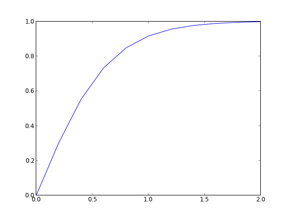
plt.plot(X, Y)
plt.savefig('images/bvp-nonlinear-1.png')

That code looks useful, so I put it in the pycse module in the function BVP_nl. Here is an example usage. We have to create two functions, one for the differential equation, and one for the initial guess.

from pycse import  BVP_nl
import matplotlib.pyplot as plt

def Ypp(x, y, yprime):
    '''define y'' = 3*y*y' '''
    return -3.0 * y * yprime

def init(x):
    return alpha + (beta - alpha) / (x2 - x1) * x

x1 = 0.0
x2 = 2.0

alpha = 0.0
beta = 1.0

N = 11
x, y = BVP_nl(Ypp, x1, x2, alpha, beta, init, N)

plt.plot(x, y)
plt.savefig('images/bvp-nonlinear-2.png')

The results are the same.

Copyright (C) 2013 by John Kitchin. See the License for information about copying.

org-mode source

Discuss on Twitter

Transient heat conduction - partial differential equations

| categories: pde | tags: heat transfer

Matlab post adapated from http://msemac.redwoods.edu/~darnold/math55/DEproj/sp02/AbeRichards/slideshowdefinal.pdf

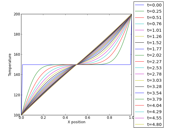
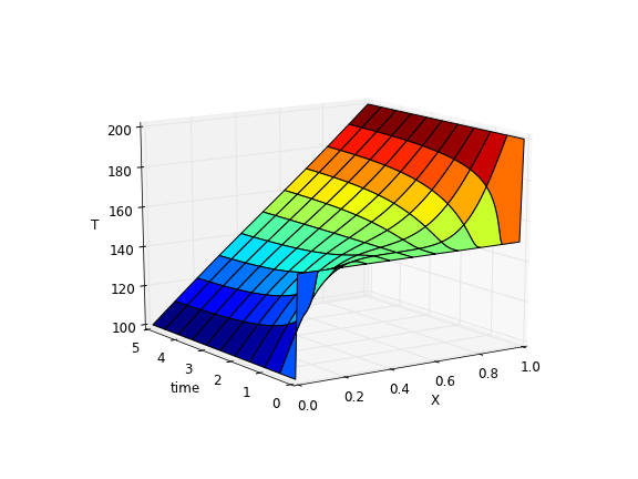
We solved a steady state BVP modeling heat conduction. Today we examine the transient behavior of a rod at constant T put between two heat reservoirs at different temperatures, again T1 = 100, and T2 = 200. The rod will start at 150. Over time, we should expect a solution that approaches the steady state solution: a linear temperature profile from one side of the rod to the other.

\(\frac{\partial u}{\partial t} = k \frac{\partial^2 u}{\partial x^2}\)

at \(t=0\), in this example we have \(u_0(x) = 150\) as an initial condition. with boundary conditions \(u(0,t)=100\) and \(u(L,t)=200\).

In Matlab there is the pdepe command. There is not yet a PDE solver in scipy. Instead, we will utilze the method of lines to solve this problem. We discretize the rod into segments, and approximate the second derivative in the spatial dimension as \(\frac{\partial^2 u}{\partial x^2} = (u(x + h) - 2 u(x) + u(x-h))/ h^2\) at each node. This leads to a set of coupled ordinary differential equations that is easy to solve.

Let us say the rod has a length of 1, \(k=0.02\), and solve for the time-dependent temperature profiles.

import numpy as np
from scipy.integrate import odeint
import matplotlib.pyplot as plt

N = 100  # number of points to discretize
L = 1.0
X = np.linspace(0, L, N) # position along the rod
h = L / (N - 1)

k = 0.02

def odefunc(u, t):
    dudt = np.zeros(X.shape)

    dudt[0] = 0 # constant at boundary condition
    dudt[-1] = 0

    # now for the internal nodes
    for i in range(1, N-1):
        dudt[i] = k * (u[i + 1] - 2*u[i] + u[i - 1]) / h**2

    return dudt

init = 150.0 * np.ones(X.shape) # initial temperature
init[0] = 100.0  # one boundary condition
init[-1] = 200.0 # the other boundary condition

tspan = np.linspace(0.0, 5.0, 100)
sol = odeint(odefunc, init, tspan)


for i in range(0, len(tspan), 5):
    plt.plot(X, sol[i], label='t={0:1.2f}'.format(tspan[i]))

# put legend outside the figure
plt.legend(loc='center left', bbox_to_anchor=(1, 0.5))
plt.xlabel('X position')
plt.ylabel('Temperature')

# adjust figure edges so the legend is in the figure
plt.subplots_adjust(top=0.89, right=0.77)
plt.savefig('images/pde-transient-heat-1.png')


# Make a 3d figure
from mpl_toolkits.mplot3d import Axes3D
fig = plt.figure()
ax = fig.add_subplot(111, projection='3d')

SX, ST = np.meshgrid(X, tspan)
ax.plot_surface(SX, ST, sol, cmap='jet')
ax.set_xlabel('X')
ax.set_ylabel('time')
ax.set_zlabel('T')
ax.view_init(elev=15, azim=-124) # adjust view so it is easy to see
plt.savefig('images/pde-transient-heat-3d.png')

# animated solution. We will use imagemagick for this

# we save each frame as an image, and use the imagemagick convert command to 
# make an animated gif
for i in range(len(tspan)):
    plt.clf()
    plt.plot(X, sol[i])
    plt.xlabel('X')
    plt.ylabel('T(X)')
    plt.title('t = {0}'.format(tspan[i]))
    plt.savefig('___t{0:03d}.png'.format(i))

import commands
print commands.getoutput('convert -quality 100 ___t*.png images/transient_heat.gif')
print commands.getoutput('rm ___t*.png') #remove temp files


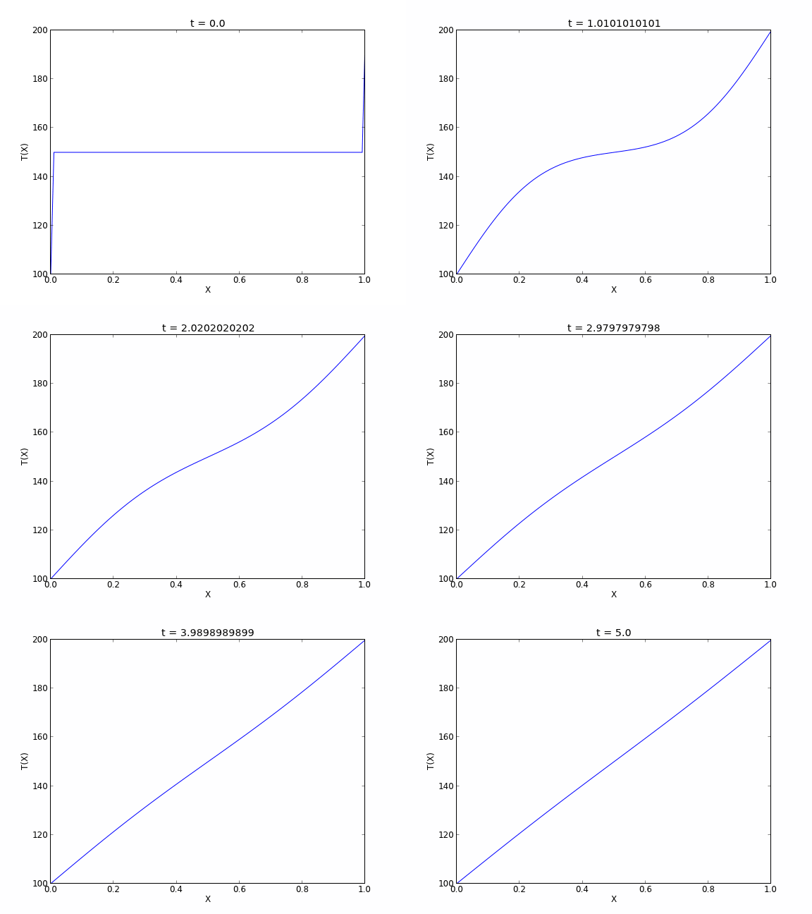
This version of the graphical solution is not that easy to read, although with some study you can see the solution evolves from the initial condition which is flat, to the steady state solution which is a linear temperature ramp.

The 3d version may be easier to interpret. The temperature profile starts out flat, and gradually changes to the linear ramp.

Finally, the animated solution.

Copyright (C) 2013 by John Kitchin. See the License for information about copying.

org-mode source
Discuss on Twitter

Another approach to error propagation

| categories: statistics | tags:

In the previous section we examined an analytical approach to error propagation, and a simulation based approach. There is another approach to error propagation, using the uncertainties module (https://pypi.python.org/pypi/uncertainties/). You have to install this package, e.g. pip install uncertainties. After that, the module provides new classes of numbers and functions that incorporate uncertainty and propagate the uncertainty through the functions. In the examples that follow, we repeat the calculations from the previous section using the uncertainties module.

Addition and subtraction

import uncertainties as u

A = u.ufloat((2.5, 0.4))
B = u.ufloat((4.1, 0.3))
print A + B
print A - B
>>> >>> >>> 6.6+/-0.5
-1.6+/-0.5

Multiplication and division

F = u.ufloat((25, 1))
x = u.ufloat((6.4, 0.4))

t = F * x
print t

d = F / x
print d
>>> >>> >>> 160.0+/-11.8726576637
>>> >>> 3.90625+/-0.289859806243

Exponentiation

t = u.ufloat((2.03, 0.0203))
print t**5

from uncertainties.umath import sqrt
A = u.ufloat((16.07, 0.06))
print sqrt(A)
# print np.sqrt(A) # this does not work

from uncertainties import unumpy as unp
print unp.sqrt(A)
34.4730881243+/-1.72365440621
>>> >>> >>> >>> 4.00874045057+/-0.00748364738749
... >>> >>> 4.00874045057+/-0.00748364738749

Note in the last example, we had to either import a function from uncertainties.umath or import a special version of numpy that handles uncertainty. This may be a limitation of teh uncertainties package as not all functions in arbitrary modules can be covered. Note, however, that you can wrap a function to make it handle uncertainty like this.

import numpy as np

wrapped_sqrt = u.wrap(np.sqrt)
print wrapped_sqrt(A)
>>> >>> 4.00874045057+/-0.00748364738774

Propagation of errors in an integral

import numpy as np
import uncertainties as u

x = np.array([u.ufloat((1, 0.01)), 
              u.ufloat((2, 0.1)),
              u.ufloat((3, 0.1))])

y = 2 * x

print np.trapz(x, y)
>>> >>> ... ... >>> >>> >>> >>> 8.0+/-0.600333240792

Chain rule in error propagation

v0 = u.ufloat((1.2, 0.02))
a = u.ufloat((3.0, 0.3))
t = u.ufloat((12.0, 0.12))

v = v0 + a * t
print v
>>> >>> >>> >>> 37.2+/-3.61801050303

A real example? This is what I would setup for a real working example. We try to compute the exit concentration from a CSTR. The idea is to wrap the “external” fsolve function using the uncertainties.wrap function, which handles the units. Unfortunately, it does not work, and it is not clear why. But see the following discussion for a fix.

from scipy.optimize import fsolve

Fa0 = u.ufloat((5.0, 0.05))
v0 = u.ufloat((10., 0.1))

V = u.ufloat((66000.0, 100))  # reactor volume L^3
k = u.ufloat((3.0, 0.2))      # rate constant L/mol/h

def func(Ca):
    "Mole balance for a CSTR. Solve this equation for func(Ca)=0"
    Fa = v0 * Ca     # exit molar flow of A
    ra = -k * Ca**2  # rate of reaction of A L/mol/h
    return Fa0 - Fa + V * ra

# CA guess that that 90 % is reacted away
CA_guess = 0.1 * Fa0 / v0

wrapped_fsolve = u.wrap(fsolve)
CA_sol = wrapped_fsolve(func, CA_guess)

print 'The exit concentration is {0} mol/L'.format(CA_sol)
>>> >>> >>> >>> >>> >>> >>> ... ... ... ... ... >>> ... >>> >>> >>> <function fsolve at 0x148f25f0>
>>> >>> The exit concentration is NotImplemented mol/L

I got a note from the author of the uncertainties package explaining the cryptic error above, and a solution for it. The error arises because fsolve does not know how to deal with uncertainties. The idea is to create a function that returns a float, when everything is given as a float. Then, we wrap the fsolve call, and finally wrap the wrapped fsolve call!

  • Step 1. Write the function to solve with arguments for all unitted quantities. This function may be called with uncertainties, or with floats.
  • Step 2. Wrap the call to fsolve in a function that takes all the parameters as arguments, and that returns the solution.
  • Step 3. Use uncertainties.wrap to wrap the function in Step 2 to get the answer with uncertainties.

Here is the code that does work:

import uncertainties as u
from scipy.optimize import fsolve

Fa0 = u.ufloat((5.0, 0.05))
v0 = u.ufloat((10., 0.1))

V = u.ufloat((66000.0, 100.0))  # reactor volume L^3
k = u.ufloat((3.0, 0.2))      # rate constant L/mol/h

# Step 1
def func(Ca, v0, k, Fa0, V):
    "Mole balance for a CSTR. Solve this equation for func(Ca)=0"
    Fa = v0 * Ca     # exit molar flow of A
    ra = -k * Ca**2  # rate of reaction of A L/mol/h
    return Fa0 - Fa + V * ra

# Step 2
def Ca_solve(v0, k, Fa0, V): 
    'wrap fsolve to pass parameters as float or units'
    # this line is a little fragile. You must put [0] at the end or
    # you get the NotImplemented result
    sol = fsolve(func, 0.1 * Fa0 / v0, args=(v0, k, Fa0, V))[0]
    return sol

# Step 3
print u.wrap(Ca_solve)(v0, k, Fa0, V)
0.005+/-0.000167764327667

It would take some practice to get used to this, but the payoff is that you have an “automatic” error propagation method.

Being ever the skeptic, let us compare the result above to the Monte Carlo approach to error estimation below.

import numpy as np
from scipy.optimize import fsolve

N = 10000
Fa0 = np.random.normal(5, 0.05, (1, N))
v0 = np.random.normal(10.0, 0.1, (1, N))
V =  np.random.normal(66000, 100, (1,N))
k = np.random.normal(3.0, 0.2, (1, N))

SOL = np.zeros((1, N))

for i in range(N):
    def func(Ca):
        return Fa0[0,i] - v0[0,i] * Ca + V[0,i] * (-k[0,i] * Ca**2)
    SOL[0,i] = fsolve(func, 0.1 * Fa0[0,i] / v0[0,i])[0]

print 'Ca(exit) = {0}+/-{1}'.format(np.mean(SOL), np.std(SOL))
Ca(exit) = 0.00500829453185+/-0.000169103578901

I am pretty content those are the same!

1 Summary

The uncertainties module is pretty amazing. It automatically propagates errors through a pretty broad range of computations. It is a little tricky for third-party packages, but it seems doable.

Read more about the package at http://pythonhosted.org/uncertainties/index.html.

Copyright (C) 2013 by John Kitchin. See the License for information about copying.

org-mode source
Discuss on Twitter
« Previous Page -- Next Page »